Bellman Ford’s Algorithm in Data Structures - Working, Example and Applications

Bellman Ford’s Algorithm in Data Structures: An Overview

The Bellman-Ford Algorithm is a powerful tool that helps us find the shortest paths in networks. This algorithm can help you understand the implications of multiple connections and how they determine efficient travel routes or optimal cost networks. In this DSA tutorial, we will explore the Bellman-Ford Algorithm to get a better understanding of its basic principles and practical applications.

To further enhance your understanding and application of Bellman Ford's Algorithm, consider enrolling in the Best Data Structures And Algorithms Course, to gain comprehensive insights into effective data structure utilization for improved problem-solving and time management.

What is Bellman Ford's Algorithm in Data Structures?

Bellman-Ford algorithm is used to calculate the shortest paths from a single source vertex to all vertices in the graph.This algorithm even works on graphs with a negative edge weight cycle i.e. a cycle of edges with the sum of weights equal to a negative number. This algorithm follows the bottom-up approach.

At its core, the algorithm works by building up a set of "distance estimates" for each node in a graph, gradually refining them until every node has the best possible estimate. While the algorithm may seem complex at first glance, its ability to solve a wide variety of problems has made it a crucial tool for many fields, from computer science to civil engineering.

Bellman Ford's Algorithm Example

Here's an example of the bellman ford's algorithm in action:

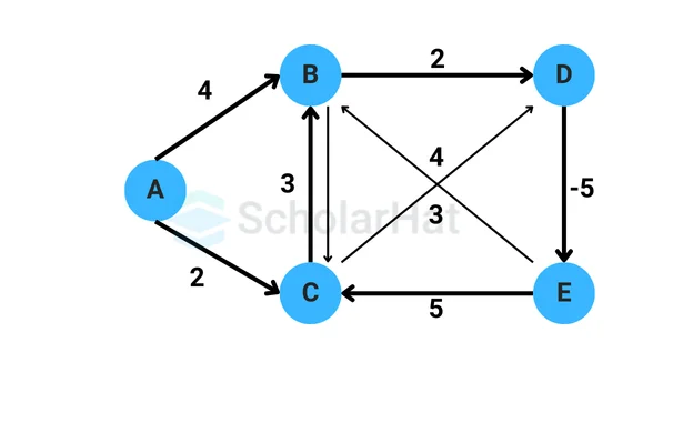
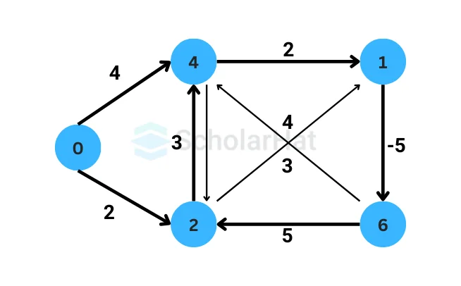
Let's consider a directed weighted graph with the following edges and their respective weights:

• Edge 1: A -> B, weight = 2
• Edge 2: A -> C, weight = 4
• Edge 3: B -> C, weight = 1
• Edge 4: B -> D, weight = 7
• Edge 5: C -> D, weight = 3
• Edge 6: D -> A, weight = 5

We want to find the shortest paths from a source vertex (let's say A) to all other vertices in the graph.

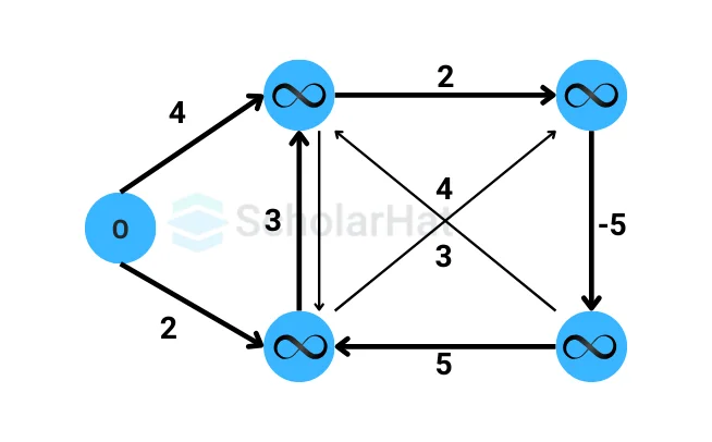
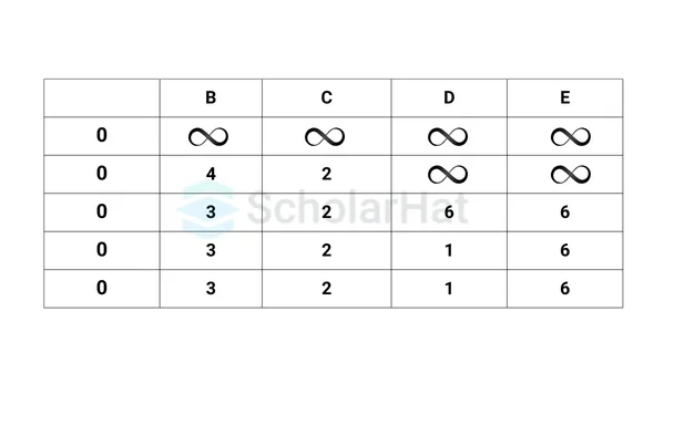
Step 1: Initialization

We set the distance to the source vertex as 0, and all other distances as infinity.

• Distance to A: 0
• Distance to B: Infinity
• Distance to C: Infinity
• Distance to D: Infinity

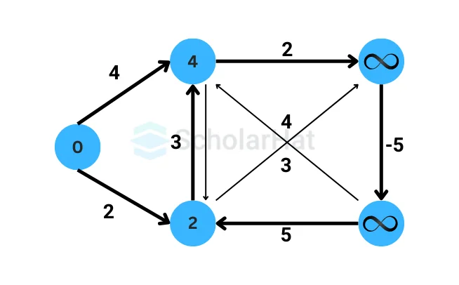
Step 2: Relaxation

We iterate over all the edges |V| - 1 time, where |V| is the number of vertices in the graph, and relax the edges. In each iteration, we update the distances if we find a shorter path.

Iteration 1:

• Distance to A: 0
• Distance to B: 2
• Distance to C: 4
• Distance to D: Infinity

Iteration 2:

• Distance to A: 0
• Distance to B: 2
• Distance to C: 3
• Distance to D: 6

Iteration 3:

• Distance to A: 0
• Distance to B: 2
• Distance to C: 3
• Distance to D: 6

Iteration 4:

• Distance to A: 0
• Distance to B: 2
• Distance to C: 3
• Distance to D: 6

Iteration 5:

• Distance to A: 0
• Distance to B: 2
• Distance to C: 3
• Distance to D: 6

Step 3: Negative cycle detection

After |V| - 1 iterations, we check for any negative cycles in the graph. In this example, there are no negative cycles.

Step 4: Result

The final distances from the source vertex A to all other vertices are as follows:

• Distance to A: 0
• Distance to B: 2
• Distance to C: 3
• Distance to D: 6

So, the shortest path from A to B is 2, from A to C is 3, and from A to D is 6.

Read More - Data Structure Interview Questions and Answers

How Bellman Ford's Algorithm Works?

Bellman-Ford's algorithm is a shortest path algorithm used to find the shortest paths from a source vertex to all other vertices in a weighted directed graph. It can handle graphs with negative edge weights, unlike Dijkstra's algorithm, which requires non-negative weights. The algorithm works as follows:

1. Initialize the distance values for all vertices in the graph as infinity, except for the source vertex, which is set to 0. Also, initialize the predecessor of all vertices as undefined.

   Relaxation step: Repeat the following process |V|-1 times, where |V| is the number of vertices in the graph.

   

2. For each edge (u, v) in the graph, where u is the source vertex and v is the destination vertex:
   • If the distance from the source vertex to u plus the weight of the edge (u, v) is less than the current distance value of v, update the distance of v with this new value.
   • Also, update the predecessor of v as u.

   

3. Check for negative-weight cycles: Repeat the following process for each edge (u, v) in the graph.
   • If the distance from the source vertex to u plus the weight of the edge (u, v) is less than the current distance value of v, then there is a negative-weight cycle in the graph.

   

4. After completing the relaxation step |V|-1 times, the algorithm will have calculated the shortest distances from the source vertex to all other vertices in the graph (if no negative-weight cycles exist). If there is a negative-weight cycle, step 3 will detect it.

   

5. If required, the shortest paths can be reconstructed using the predecessor information. Starting from the destination vertex, follow the predecessor pointers until reaching the source vertex to obtain the shortest path.

   

The algorithm guarantees the correct shortest path distances if there are no negative-weight cycles reachable from the source vertex. However, if there is a negative-weight cycle that can be reached from the source vertex, the algorithm will detect it in step 3. In such cases, the algorithm cannot provide meaningful shortest path distances, as the negative-weight cycle allows for infinite negative weight reductions

Bellman Ford's Algorithm Pseudocode

Bellman Ford's algorithm, is used to find the shortest paths from a single source vertex to all other vertices in a weighted directed graph. The algorithm can handle negative edge weights but detects negative cycles.

function BellmanFord(Graph, source):
   // Step 1: Initialization
   for each vertex v in Graph:
     distance[v] := infinity
     predecessor[v] := null
   distance[source] := 0
 
   // Step 2: Relaxation
   for i from 1 to |V|-1:
     for each edge (u, v) in Graph:
       if distance[u] + weight(u, v) < distance[v]:
         distance[v] := distance[u] + weight(u, v)
         predecessor[v] := u
 
   // Step 3: Check for negative cycles
   for each edge (u, v) in Graph:
     if distance[u] + weight(u, v) < distance[v]:
       return "Graph contains a negative cycle"
 
   // Step 4: Output the shortest paths
   return distance[], predecessor[]

In this pseudocode:

• The graphrepresents the input graph.
• The source is the source vertex from which to find the shortest paths.
• distance[v] represents the shortest distance from the source to vertex v.
• predecessor[v] stores the predecessor of vertex v in the shortest path.

The algorithm consists of four main steps:

1. Initialization: Set the distance of all vertices to infinity, except for the source vertex, which is set to 0. Set the predecessor of all vertices to null.
2. Relaxation: Perform a relaxation step for each edge in the graph |V|-1 times. The relaxation step updates the distance to each vertex v if there exists a shorter path through vertex u.
3. Check for negative cycles: Perform one more iteration to check for negative cycles. If a shorter path can still be found, then there exists a negative cycle in the graph.
4. Output the shortest paths: After completing the algorithm, the shortest distances and predecessors are returned.

Note that |V| represents the number of vertices in the graph, and weight(u, v) returns the weight/cost of the edge (u, v).

Implementation of Bellman Ford’s Algorithm

class Graph:

	def __init__(self, vertices):
		self.V = vertices # No. of vertices
		self.graph = []

	# function to add an edge to graph
	def addEdge(self, u, v, w):
		self.graph.append([u, v, w])

	# utility function used to print the solution
	def printArr(self, dist):
		print("Vertex Distance from Source")
		for i in range(self.V):
			print("{0}\t\t{1}".format(i, dist[i]))

	# The main function that finds shortest distances from src to
	# all other vertices using Bellman-Ford algorithm. The function
	# also detects negative weight cycle
	def BellmanFord(self, src):

		# Step 1: Initialize distances from src to all other vertices
		# as INFINITE
		dist = [float("Inf")] * self.V
		dist[src] = 0

		# Step 2: Relax all edges |V| - 1 times. A simple shortest
		# path from src to any other vertex can have at-most |V| - 1
		# edges
		for _ in range(self.V - 1):
			# Update dist value and parent index of the adjacent vertices of
			# the picked vertex. Consider only those vertices which are still in
			# queue
			for u, v, w in self.graph:
				if dist[u] != float("Inf") and dist[u] + w < dist[v]:
					dist[v] = dist[u] + w

		# Step 3: check for negative-weight cycles. The above step
		# guarantees shortest distances if graph doesn't contain
		# negative weight cycle. If we get a shorter path, then there
		# is a cycle.

		for u, v, w in self.graph:
			if dist[u] != float("Inf") and dist[u] + w < dist[v]:
				print("Graph contains negative weight cycle")
				return

		# print all distance
		self.printArr(dist)


# Driver's code
if __name__ == '__main__':
	g = Graph(5)
	g.addEdge(0, 1, -1)
	g.addEdge(0, 2, 4)
	g.addEdge(1, 2, 3)
	g.addEdge(1, 3, 2)
	g.addEdge(1, 4, 2)
	g.addEdge(3, 2, 5)
	g.addEdge(3, 1, 1)
	g.addEdge(4, 3, -3)

	# function call
	g.BellmanFord(0)
 

import java.io.*;
import java.lang.*;
import java.util.*;

// A class to represent a connected, directed and weighted
// graph
class Graph {

	// A class to represent a weighted edge in graph
	class Edge {
		int src, dest, weight;
		Edge() { src = dest = weight = 0; }
	};

	int V, E;
	Edge edge[];

	// Creates a graph with V vertices and E edges
	Graph(int v, int e)
	{
		V = v;
		E = e;
		edge = new Edge[e];
		for (int i = 0; i < e; ++i)
			edge[i] = new Edge();
	}

	// The main function that finds shortest distances from
	// src to all other vertices using Bellman-Ford
	// algorithm. The function also detects negative weight
	// cycle
	void BellmanFord(Graph graph, int src)
	{
		int V = graph.V, E = graph.E;
		int dist[] = new int[V];

		// Step 1: Initialize distances from src to all
		// other vertices as INFINITE
		for (int i = 0; i < V; ++i)
			dist[i] = Integer.MAX_VALUE;
		dist[src] = 0;

		// Step 2: Relax all edges |V| - 1 times. A simple
		// shortest path from src to any other vertex can
		// have at-most |V| - 1 edges
		for (int i = 1; i < V; ++i) {
			for (int j = 0; j < E; ++j) {
				int u = graph.edge[j].src;
				int v = graph.edge[j].dest;
				int weight = graph.edge[j].weight;
				if (dist[u] != Integer.MAX_VALUE
					&& dist[u] + weight < dist[v])
					dist[v] = dist[u] + weight;
			}
		}

		// Step 3: check for negative-weight cycles. The
		// above step guarantees shortest distances if graph
		// doesn't contain negative weight cycle. If we get
		// a shorter path, then there is a cycle.
		for (int j = 0; j < E; ++j) {
			int u = graph.edge[j].src;
			int v = graph.edge[j].dest;
			int weight = graph.edge[j].weight;
			if (dist[u] != Integer.MAX_VALUE
				&& dist[u] + weight < dist[v]) {
				System.out.println(
					"Graph contains negative weight cycle");
				return;
			}
		}
		printArr(dist, V);
	}

	// A utility function used to print the solution
	void printArr(int dist[], int V)
	{
		System.out.println("Vertex Distance from Source");
		for (int i = 0; i < V; ++i)
			System.out.println(i + "\t\t" + dist[i]);
	}

	// Driver's code
	public static void main(String[] args)
	{
		int V = 5; // Number of vertices in graph
		int E = 8; // Number of edges in graph

		Graph graph = new Graph(V, E);

		// add edge 0-1 (or A-B in above figure)
		graph.edge[0].src = 0;
		graph.edge[0].dest = 1;
		graph.edge[0].weight = -1;

		// add edge 0-2 (or A-C in above figure)
		graph.edge[1].src = 0;
		graph.edge[1].dest = 2;
		graph.edge[1].weight = 4;

		// add edge 1-2 (or B-C in above figure)
		graph.edge[2].src = 1;
		graph.edge[2].dest = 2;
		graph.edge[2].weight = 3;

		// add edge 1-3 (or B-D in above figure)
		graph.edge[3].src = 1;
		graph.edge[3].dest = 3;
		graph.edge[3].weight = 2;

		// add edge 1-4 (or B-E in above figure)
		graph.edge[4].src = 1;
		graph.edge[4].dest = 4;
		graph.edge[4].weight = 2;

		// add edge 3-2 (or D-C in above figure)
		graph.edge[5].src = 3;
		graph.edge[5].dest = 2;
		graph.edge[5].weight = 5;

		// add edge 3-1 (or D-B in above figure)
		graph.edge[6].src = 3;
		graph.edge[6].dest = 1;
		graph.edge[6].weight = 1;

		// add edge 4-3 (or E-D in above figure)
		graph.edge[7].src = 4;
		graph.edge[7].dest = 3;
		graph.edge[7].weight = -3;
		
		// Function call
		graph.BellmanFord(graph, 0);
	}
}
    

#include <iostream>
using namespace std;

// a structure to represent a weighted edge in graph
struct Edge {
	int src, dest, weight;
};

// a structure to represent a connected, directed and
// weighted graph
struct Graph {
	// V-> Number of vertices, E-> Number of edges
	int V, E;

	// graph is represented as an array of edges.
	struct Edge* edge;
};

// Creates a graph with V vertices and E edges
struct Graph* createGraph(int V, int E)
{
	struct Graph* graph = new Graph;
	graph->V = V;
	graph->E = E;
	graph->edge = new Edge[E];
	return graph;
}

// A utility function used to print the solution
void printArr(int dist[], int n)
{
	printf("Vertex Distance from Source\n");
	for (int i = 0; i < n; ++i)
		printf("%d \t\t %d\n", i, dist[i]);
}

// The main function that finds shortest distances from src
// to all other vertices using Bellman-Ford algorithm. The
// function also detects negative weight cycle
void BellmanFord(struct Graph* graph, int src)
{
	int V = graph->V;
	int E = graph->E;
	int dist[V];

	// Step 1: Initialize distances from src to all other
	// vertices as INFINITE
	for (int i = 0; i < V; i++)
		dist[i] = INT_MAX;
	dist[src] = 0;

	// Step 2: Relax all edges |V| - 1 times. A simple
	// shortest path from src to any other vertex can have
	// at-most |V| - 1 edges
	for (int i = 1; i <= V - 1; i++) {
		for (int j = 0; j < E; j++) {
			int u = graph->edge[j].src;
			int v = graph->edge[j].dest;
			int weight = graph->edge[j].weight;
			if (dist[u] != INT_MAX
				&& dist[u] + weight < dist[v])
				dist[v] = dist[u] + weight;
		}
	}

	// Step 3: check for negative-weight cycles. The above
	// step guarantees shortest distances if graph doesn't
	// contain negative weight cycle. If we get a shorter
	// path, then there is a cycle.
	for (int i = 0; i < E; i++) {
		int u = graph->edge[i].src;
		int v = graph->edge[i].dest;
		int weight = graph->edge[i].weight;
		if (dist[u] != INT_MAX
			&& dist[u] + weight < dist[v]) {
			printf("Graph contains negative weight cycle");
			return; // If negative cycle is detected, simply
					// return
		}
	}

	printArr(dist, V);

	return;
}

// Driver's code
int main()
{
	/* Let us create the graph given in above example */
	int V = 5; // Number of vertices in graph
	int E = 8; // Number of edges in graph
	struct Graph* graph = createGraph(V, E);

	// add edge 0-1 (or A-B in above figure)
	graph->edge[0].src = 0;
	graph->edge[0].dest = 1;
	graph->edge[0].weight = -1;

	// add edge 0-2 (or A-C in above figure)
	graph->edge[1].src = 0;
	graph->edge[1].dest = 2;
	graph->edge[1].weight = 4;

	// add edge 1-2 (or B-C in above figure)
	graph->edge[2].src = 1;
	graph->edge[2].dest = 2;
	graph->edge[2].weight = 3;

	// add edge 1-3 (or B-D in above figure)
	graph->edge[3].src = 1;
	graph->edge[3].dest = 3;
	graph->edge[3].weight = 2;

	// add edge 1-4 (or B-E in above figure)
	graph->edge[4].src = 1;
	graph->edge[4].dest = 4;
	graph->edge[4].weight = 2;

	// add edge 3-2 (or D-C in above figure)
	graph->edge[5].src = 3;
	graph->edge[5].dest = 2;
	graph->edge[5].weight = 5;

	// add edge 3-1 (or D-B in above figure)
	graph->edge[6].src = 3;
	graph->edge[6].dest = 1;
	graph->edge[6].weight = 1;

	// add edge 4-3 (or E-D in above figure)
	graph->edge[7].src = 4;
	graph->edge[7].dest = 3;
	graph->edge[7].weight = -3;
	
	// Function call
	BellmanFord(graph, 0);

	return 0;
}
    

Output

Vertex Distance from Source
0		0
1		-1
2		2
3		-2
4		1

Applications of Bellman Ford's Algorithm

1. Routing protocols: The Bellman-Ford algorithm is widely used in computer networks as the basis for distance-vector routing protocols. These protocols are responsible for determining the best path for data packets to travel through a network. Examples of routing protocols that use the Bellman-Ford algorithm include the Routing Information Protocol (RIP) and the Border Gateway Protocol (BGP).
2. Network topology analysis: The Bellman-Ford algorithm can be used to analyze and understand the topology of a network. By running the algorithm on a network graph, it can determine the shortest path and associated costs between different nodes. This information is valuable for network administrators to optimize network performance and identify potential bottlenecks.
3. Internet Service Providers (ISPs): ISPs use the Bellman-Ford algorithm for network traffic engineering and to ensure efficient routing of data across their networks. By applying the algorithm to the network topology, ISPs can determine the best path for data packets to reach their destination, considering factors such as link capacities, congestion, and network policies.
4. Distance vector protocols in wireless sensor networks: Wireless sensor networks often have limited resources, such as battery power and computing capabilities. The Bellman-Ford algorithm can be implemented in these networks to compute the shortest path while considering energy constraints and other network-specific requirements.
5. Virtual Private Networks (VPNs): The Bellman-Ford algorithm is used in VPNs to determine the optimal path for network traffic between different nodes in the VPN infrastructure. It helps establish secure and efficient communication between geographically distributed networks.
6. Resource allocation in cloud computing: The Bellman-Ford algorithm can be used to allocate resources in cloud computing environments. By modeling the cloud infrastructure as a graph, the algorithm can find the shortest path and associated costs between different resources, such as servers, storage, and network components. This information can assist in optimizing resource allocation and load balancing.

Complexity Analysis of Bellman Ford's Algorithm

1. Time Complexity

   Case	Time Complexity
   Best Case	O(E)
   Average Case	O(VE)
   Worst Case	O(VE)

2. Space Complexity: The space complexity of Bellman Ford's Algorithm is O(V).

Summary

The Bellman-Ford Algorithm is a fundamental algorithm used to find the shortest paths in a graph, considering the weights or costs associated with each edge. It is commonly used in computer networks and routing protocols. Overall, the Bellman-Ford Algorithm is a versatile and widely used algorithm for solving shortest-path problems in various domains, enabling efficient routing and resource allocation in networks.