


02
JulBreadth First Traversal and Depth First Traversal in Data Structure
23 Sep 2025
Advanced
38.2K Views
33 min read

Learn with an interactive course and practical hands-on labs
Free DSA Online Course with Certification
BFS and DFS in Data Structure
Breadth-first Search (BFS) and Depth First Traversal (DFS) are the two main algorithms to traverse the graph. BFS traverses breadthwise whereas DFS traverses depthwise. Both come under the category of recursive algorithms.
In this DSA tutorial, we will learn these two algorithms in detail. By 2027, 80% of coding interviews will focus on DSA skills. Ace them with our Free Data Structures and Algorithms Course today!
What is Breadth First Traversal in Data Structures?
Breadth-first Search (BFS) is a graph traversal algorithm that explores all the vertices of a graph in a breadthwise order. It means it starts at a given vertex or node and visits all the vertices at the same level before moving to the next level. It is a recursive algorithm for searching all the vertices of a graph or tree data structure.
BFS Algorithm
For the BFS implementation, we will categorize each vertex of the graph into two categories:- Visited
- Not Visited
Here's a step-by-step explanation of how the BFS algorithm works:
- Start by selecting a starting vertex or node.
- Add the starting vertex to the end of the queue.
- Mark the starting vertex as visited and add it to the visited array/list.
- While the queue is not empty, do the following steps:
- Remove the front vertex from the queue.
- Visit the removed vertex and process it.
- Enqueue all the adjacent vertices of the removed vertex that have not been visited yet.
- Mark each visited adjacent vertex as visited and add it to the visited array/list.
- Repeat step 4 until the queue is empty.
The graph might have two different disconnected parts so to make sure that we cover every vertex, we can also run the BFS algorithm on every node.
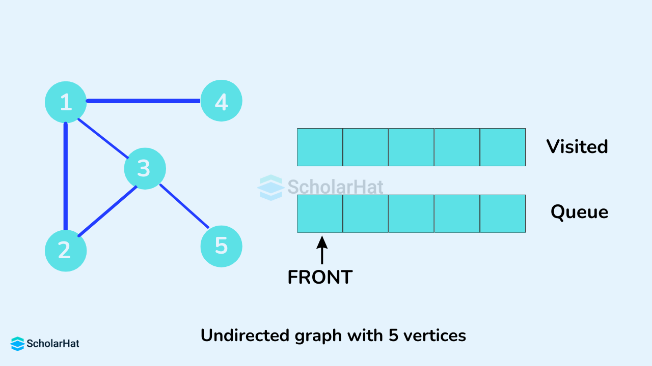
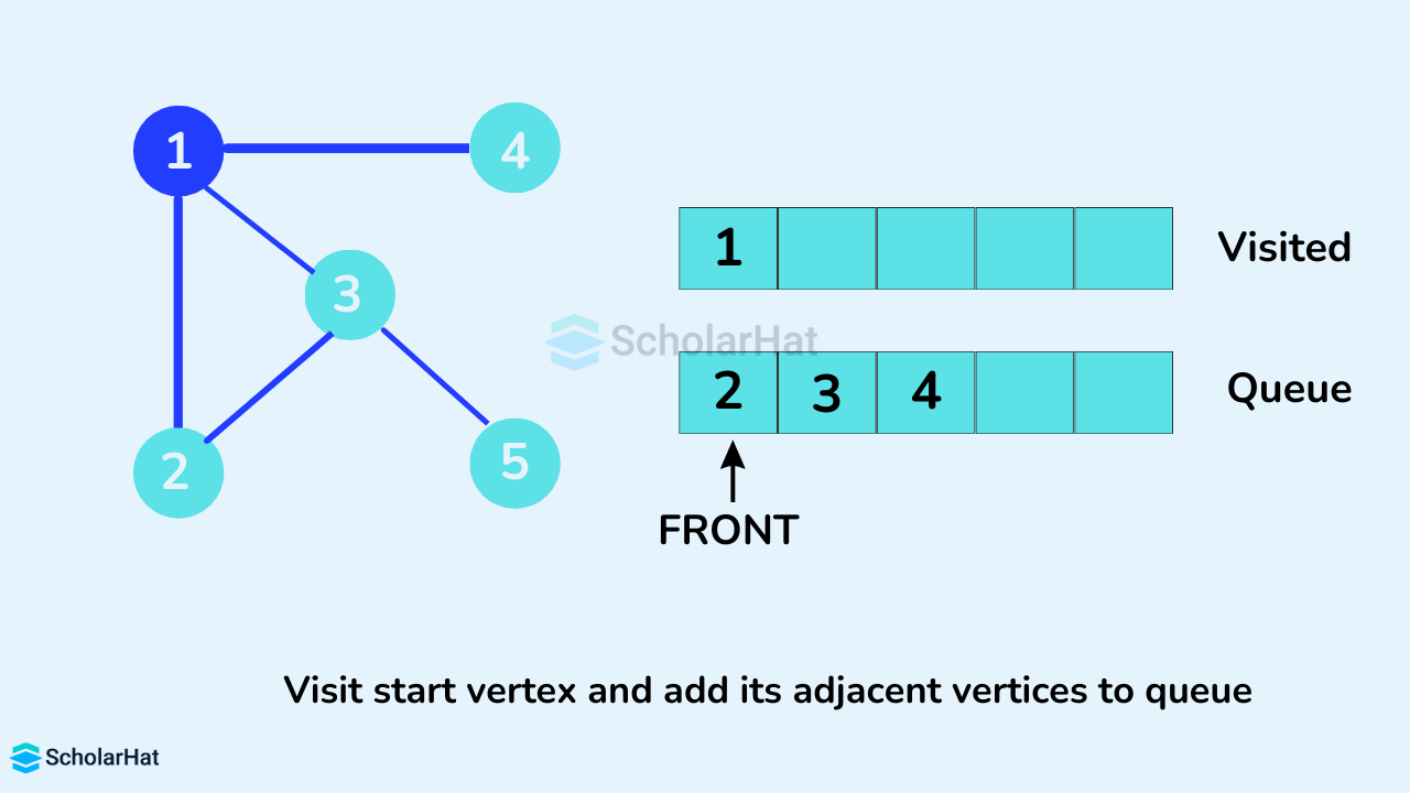
Example to illustrate the working of the BFS Algorithm
We use an undirected graph with 5 vertices.
We start from vertex 1, the BFS algorithm starts by putting it in the Visited list and putting all its adjacent vertices in the stack.
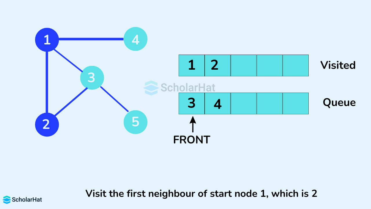
Next, we visit the element at the front of the queue i.e. 2, and go to its adjacent nodes. Since 1 has already been visited, we visit 3 instead.
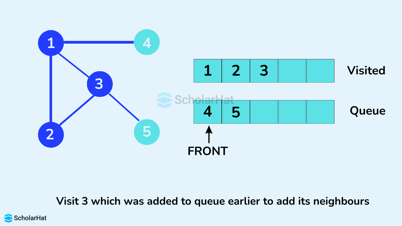
Vertex 3 has an unvisited adjacent vertex in 5, so we add that to the back of the queue and visit 4, which is at the front of the queue.
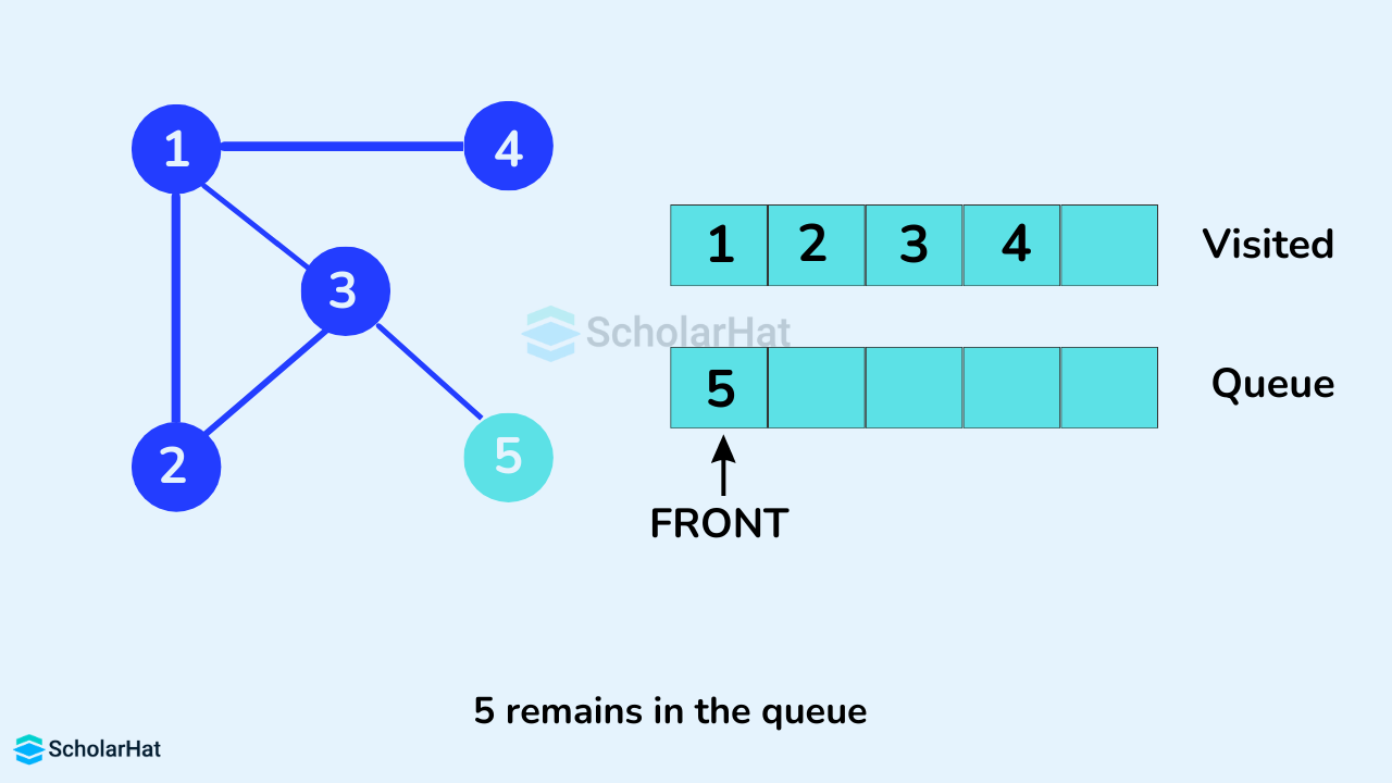
Only 5 remain in the queue since the only adjacent node of 4 i.e. 1 is already visited. We visited it.
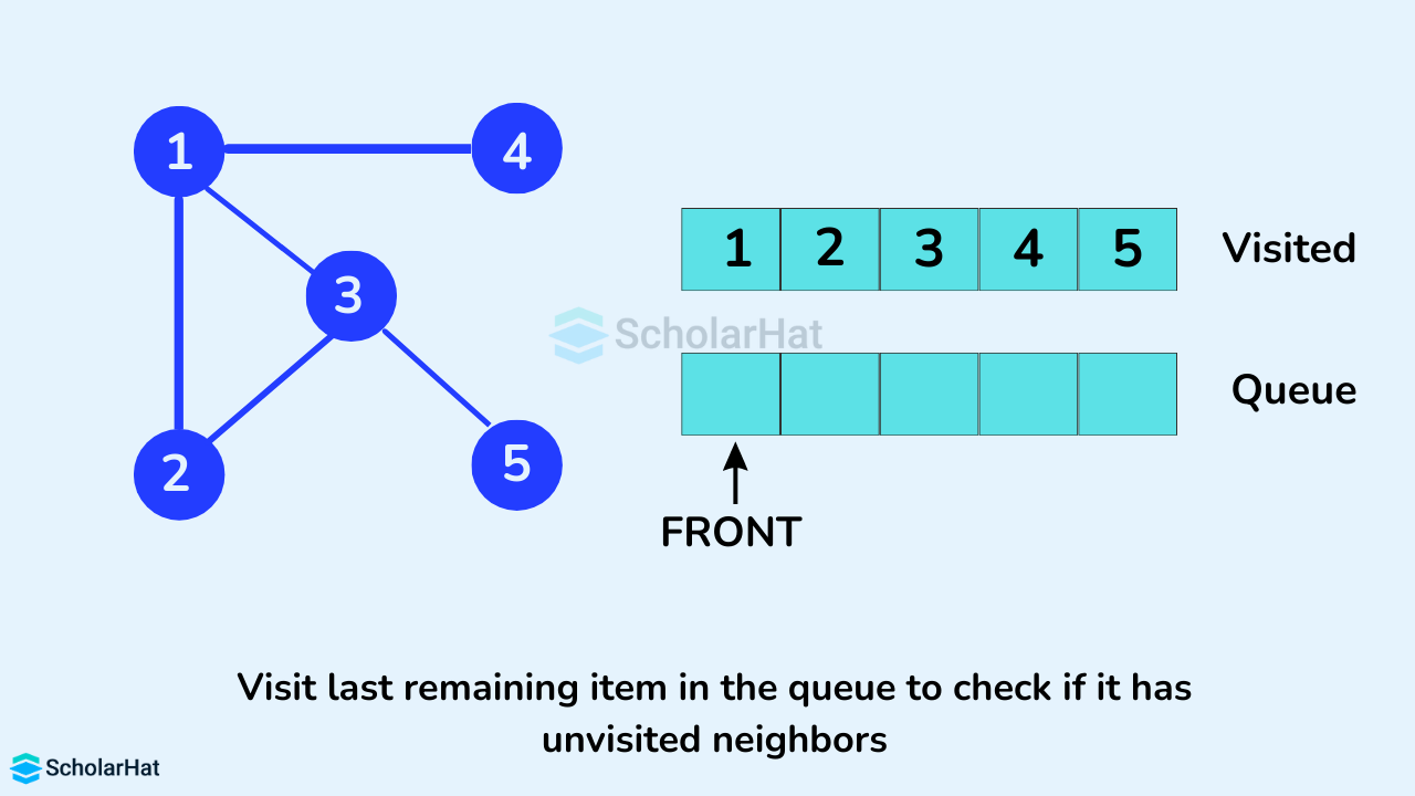
Since the queue is empty, we have completed the Breadth First Traversal of the graph.
Read More - DSA Interview Questions and Answers
Pseudocode of Breadth-First Search Algorithm
create a queue Q
mark v as visited and put v into Q
while Q is non-empty
    remove the head u of Q
    mark and enqueue all (unvisited) neighbours of u
Rules of Breadth-First Traversal Algorithm
- A Queue(which facilitates FIFO) is used in Breadth-First Search.
- Since Graphs have no root, we can start the Breadth-First Search traversal from any Vertex of the Graph.
- While Breadth-First Search, we visit all the Nodes in the Graph.
- For every Node already visited, we visit all of its unvisited neighboring Nodes and add them to the Queue.
- Breadth-First Search continues until all Vertices in the graph are visited.
- No loops are caused in Breadth-First Search, as we prevent revisiting the same Node by marking them visited.
Implementation of BFS Algorithm in Different Programming Languages
from collections import deque

class Graph:
    def __init__(self, v):
        self.V = v
        self.adj = [deque() for _ in range(v)]

    def add_edge(self, v, w):
        self.adj[v].append(w)

    def bfs(self, s):
        visited = [False] * self.V
        queue = deque()

        visited[s] = True
        queue.append(s)

        while queue:
            s = queue.popleft()
            print(s, end=" ")

            for n in self.adj[s]:
                if not visited[n]:
                    visited[n] = True
                    queue.append(n)

if __name__ == "__main__":
    graph = Graph(7)

    graph.add_edge(0, 7)
    graph.add_edge(0, 2)
    graph.add_edge(1, 3)
    graph.add_edge(1, 4)
    graph.add_edge(2, 5)
    graph.add_edge(2, 1)
    graph.add_edge(3, 6)

    print("Following is Breadth First Traversal (starting from vertex 2):")
    graph.bfs(2)
// BFS algorithm in Java

import java.util.*;

public class Main {
  private int V;
  private LinkedList adj[];

  // Create a graph
  Main(int v) {
    V = v;
    adj = new LinkedList[v];
    for (int i = 0; i < v; ++i)
      adj[i] = new LinkedList();
  }

  // Add edges to the graph
  void addEdge(int v, int w) {
    adj[v].add(w);
  }

  // BFS algorithm
  void BFS(int s) {

    boolean visited[] = new boolean[V];

    LinkedList queue = new LinkedList();

    visited[s] = true;
    queue.add(s);

    while (queue.size() != 0) {
      s = queue.poll();
      System.out.print(s + " ");

      Iterator i = adj[s].listIterator();
      while (i.hasNext()) {
        int n = i.next();
        if (!visited[n]) {
          visited[n] = true;
          queue.add(n);
        }
      }
    }
  }

  public static void main(String args[]) {
    Main graph = new Main(7);

    graph.addEdge(0, 7);
graph.addEdge(0, 2);
graph.addEdge(1, 3);
graph.addEdge(1, 4);
graph.addEdge(2, 5);
graph.addEdge(2, 1);
graph.addEdge(3, 6);

    System.out.println("Following is Breadth First Traversal " + "(starting from vertex 2)");

    graph.BFS(2);
  }
}
#include <iostream>
#include <list>
#include <queue>

class Graph {
private:
    int V;
    std::list* adj;

public:
    Graph(int v) : V(v) {
        adj = new std::list[v];
    }

    ~Graph() {
        delete[] adj;
    }

    void addEdge(int v, int w) {
        adj[v].push_back(w);
    }

    void bfs(int s) {
        bool* visited = new bool[V]{false};
        std::queue queue;

        visited[s] = true;
        queue.push(s);

        while (!queue.empty()) {
            s = queue.front();
            queue.pop();

            std::cout << s << " ";

            for (int n : adj[s]) {
                if (!visited[n]) {
                    visited[n] = true;
                    queue.push(n);
                }
            }
        }

        delete[] visited;
    }
};

int main() {
    Graph graph(7);

    graph.addEdge(0, 7);
    graph.addEdge(0, 2);
    graph.addEdge(1, 3);
    graph.addEdge(1, 4);
    graph.addEdge(2, 5);
    graph.addEdge(2, 1);
    graph.addEdge(3, 6);

    std::cout << "Following is Breadth First Traversal (starting from vertex 2):" << std::endl;
    graph.bfs(2);

    return 0;
}
Output
Following is Breadth First Traversal (starting from vertex 2):
2 5 1 3 4 6
Applications of Breadth First Search Algorithm
- Minimum spanning tree for unweighted graphs:In Breadth-First Search we can reach from any given source vertex to another vertex, with the minimum number of edges, and this principle can be used to find the minimum spanning tree which is the path covering all vertices in the shortest paths.
- Peer-to-peer networking: In Peer-to-peer networking, to find the neighboring peer from any other peer, the Breadth-First Search is used.
- Crawlers in search engines: Search engines need to crawl the internet. To do so, they can start from any source page, follow the links contained in that page in the Breadth-First Search manner, and therefore explore other pages.
- GPS navigation systems: To find locations within a given radius from any source person, we can find all neighboring locations using the Breadth-First Search, and keep on exploring until those are within the K radius.
- Broadcasting in networks: While broadcasting from any source, we find all its neighboring peers and continue broadcasting to them, and so on.
- Path Finding: To find if there is a path between 2 vertices, we can take any vertex as a source, and keep on traversing until we reach the destination vertex. If we explore all vertices reachable from the source and cannot find the destination vertex, then that means there is no path between these 2 vertices.
- Finding all reachable Nodes from a given Vertex: All vertices that are reachable from a given vertex can be found using the BFS approach in any disconnected graph. The vertices that are marked as visited in the visited array after the BFS is complete contain all those reachable vertices.
What is Depth First Traversal in Data Structures?
The depth-first search algorithm works by starting from an arbitrary node of the graph and exploring as far as possible before backtracking i.e. moving to an adjacent node until there is no unvisited adjacent node. After backtracking, it repeats the same process for all the remaining vertices which have not been visited till now. It is a recursive algorithm for searching all the vertices of a graph or tree data structure.
DFS Algorithm
For the DFS implementation, we will categorize each vertex of the graph into two categories:- Visited
- Not Visited
The reason for this division is to prevent the traversal of the same node again thus, avoiding cycles in the graph. Depth First Traversal in Data Structure uses a stack to keep track of the vertices to visit. A boolean visited array is used to mark the visited vertices.
Here's a step-by-step explanation of how the DFS algorithm works::
- Start by selecting a starting vertex or node.
- Add the starting vertex on top of a stack.
- Take the top item of the stack and add it to the visited list/array.
- Create a list of that vertex's adjacent nodes. Add the ones that aren't in the visited list to the top of the stack. Keep repeating steps 3 and 4 until the stack is empty.
The graph might have two different disconnected parts so to make sure that we cover every vertex, we can also run the BFS algorithm on every node.
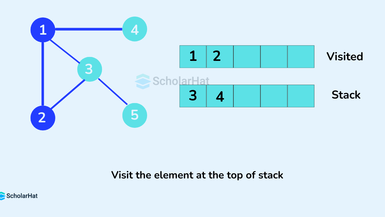
Example to illustrate the working of the DFS Algorithm
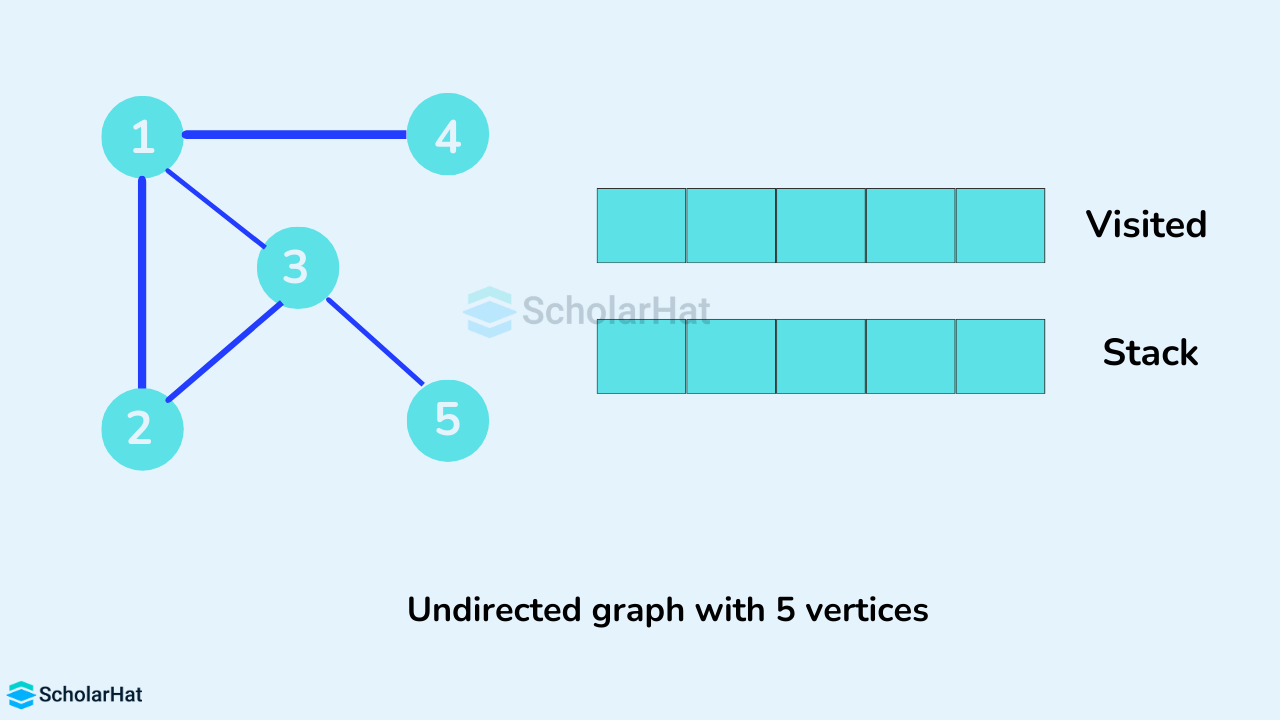
We use an undirected graph with 5 vertices.
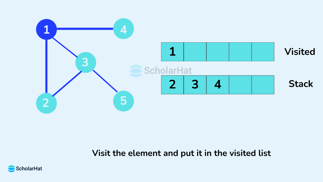
We start from vertex 1, the DFS algorithm starts by putting it in the Visited list and putting all its adjacent vertices in the stack.
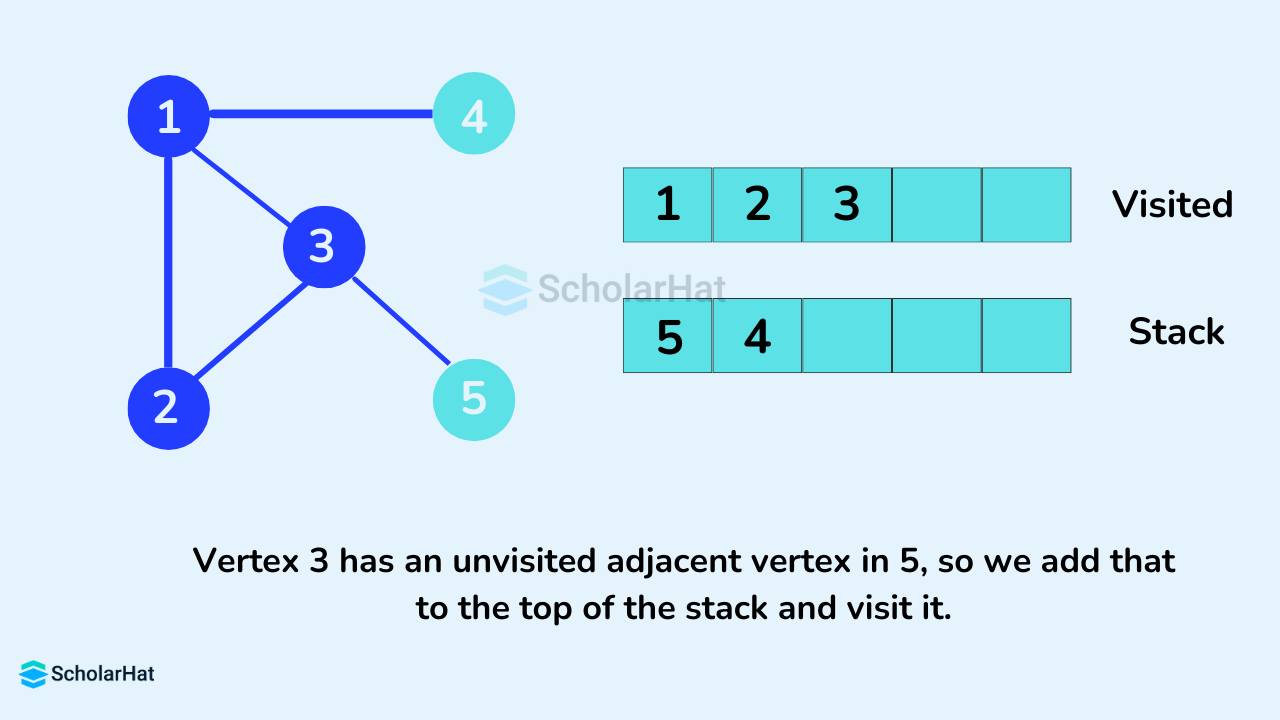
Next, we visit the element at the top of stack i.e. 2 and go to its adjacent nodes. Since 1 has already been visited, we visit 3 instead.
Vertex 3 has an unvisited adjacent vertex in 5, so we add that to the top of the stack and visit it.
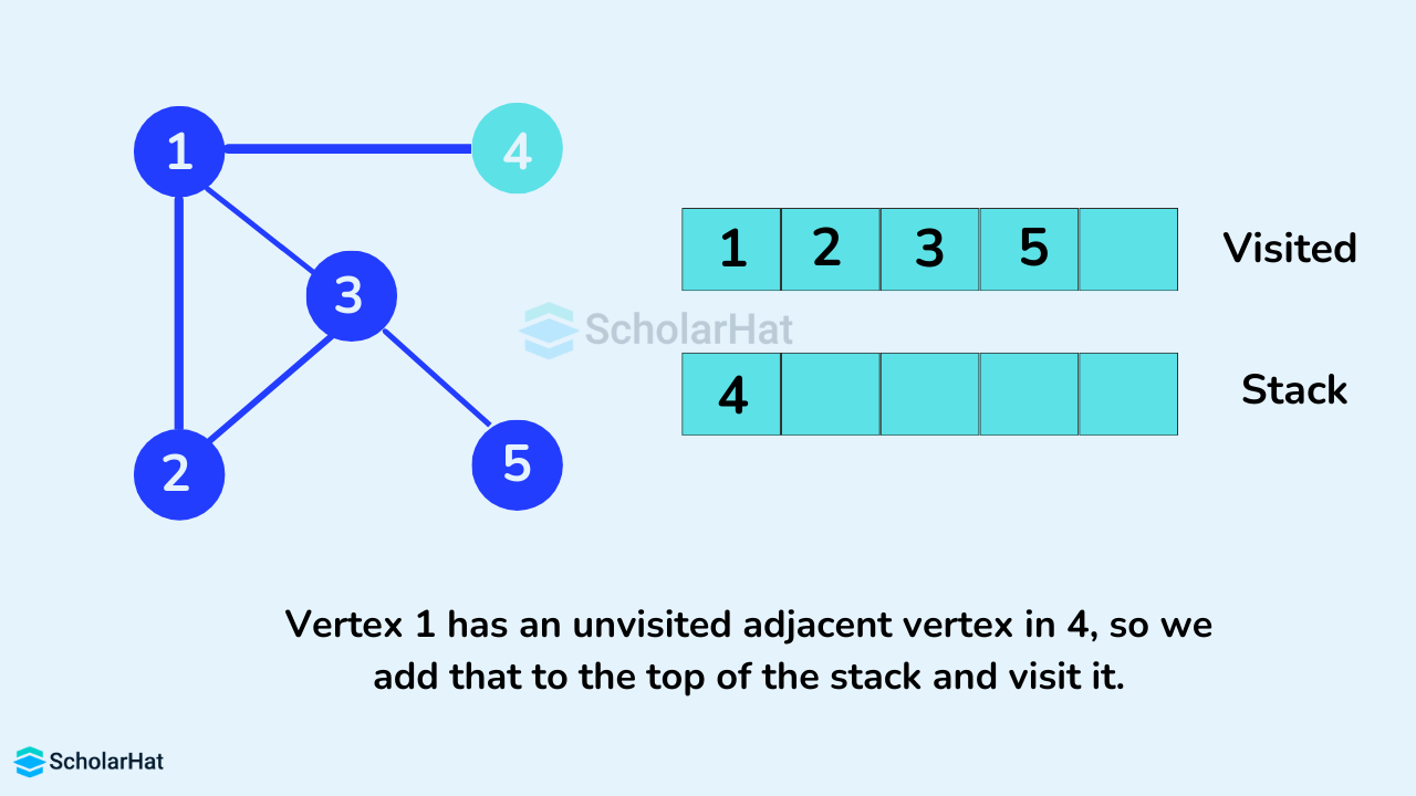
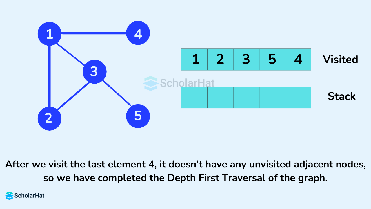
After we visit the last element 4, it doesn't have any unvisited adjacent nodes, so we have completed the Depth First Traversal of the graph.
Pseudocode of Depth-First Search Algorithm
DFS(G, u)
    u.visited = true
    for each v ∈ G.Adj[u]
        if v.visited == false
            DFS(G,v)

init() {
    For each u ∈ G
        u.visited = false
     For each u ∈ G
       DFS(G, u)
}
Implementation of DFS Algorithm in Different Programming Languages
from collections import defaultdict

class Graph:
    def __init__(self, vertices):
        self.vertices = vertices
        self.adjLists = defaultdict(list)
        self.visited = [False] * vertices

    def addEdge(self, src, dest):
        self.adjLists[src].append(dest)

    def DFS(self, vertex):
        self.visited[vertex] = True
        print(vertex, end=" ")

        for adj in self.adjLists[vertex]:
            if not self.visited[adj]:
                self.DFS(adj)

# Create a graph given
g = Graph(7)
g.addEdge(0, 7)
g.addEdge(0, 2)
g.addEdge(1, 3)
g.addEdge(1, 4)
g.addEdge(2, 5)
g.addEdge(2, 1)
g.addEdge(3, 6)

print("Following is Depth First Traversal (starting from vertex 2):")
g.DFS(2)
import java.util.*;

public class Main {
  private LinkedList adjLists[];
  private boolean visited[];

  // Graph creation
  Main(int vertices) {
    adjLists = new LinkedList[vertices];
    visited = new boolean[vertices];

    for (int i = 0; i < vertices; i++)
      adjLists[i] = new LinkedList();
  }

  // Add edges
  void addEdge(int src, int dest) {
    adjLists[src].add(dest);
  }

  // DFS algorithm
  void DFS(int vertex) {
    visited[vertex] = true;
    System.out.print(vertex + " ");

    Iterator ite = adjLists[vertex].listIterator();
    while (ite.hasNext()) {
      int adj = ite.next();
      if (!visited[adj])
        DFS(adj);
    }
  }

  public static void main(String args[]) {
    Main g = new Main(7);

   g.addEdge(0, 7);
g.addEdge(0, 2);
g.addEdge(1, 3);
g.addEdge(1, 4);
g.addEdge(2, 5);
g.addEdge(2, 1);
g.addEdge(3, 6);

    System.out.println("Following is Depth First Traversal" + "(starting from vertex 2)");

    g.DFS(2);
  }
}
#include <iostream>
#include <list>
#include <iterator>

class Graph {
private:
    int vertices;
    std::list* adjLists;
    bool* visited;

public:
    Graph(int v) : vertices(v) {
        adjLists = new std::list[v];
        visited = new bool[v]{false};
    }

    ~Graph() {
        delete[] adjLists;
        delete[] visited;
    }

    void addEdge(int src, int dest) {
        adjLists[src].push_back(dest);
    }

    void DFS(int vertex) {
        visited[vertex] = true;
        std::cout << vertex << " ";

        for (auto it = adjLists[vertex].begin(); it != adjLists[vertex].end(); ++it) {
            int adj = *it;
            if (!visited[adj])
                DFS(adj);
        }
    }
};

int main() {
    Graph g(7);

    g.addEdge(0, 7);
    g.addEdge(0, 2);
    g.addEdge(1, 3);
    g.addEdge(1, 4);
    g.addEdge(2, 5);
    g.addEdge(2, 1);
    g.addEdge(3, 6);

    std::cout << "Following is Depth First Traversal (starting from vertex 2):" << std::endl;
    g.DFS(2);

    return 0;
}
Output
Following is Depth First Traversal (starting from vertex 2):
2 5 1 3 6 4
Applications of Depth First Search Algorithm
- Finding any path between two vertices u and v in the graph.
- Finding the number of connected components present in a given undirected graph.
- For doing topological sorting of a given directed graph.
- Finding strongly connected components in the directed graph.
- Finding cycles in the given graph.
- To check if the given graph is bipartite.
Complexity Analysis of BFS and DFS Algorithms
| Time Complexity | Space Complexity | |
| BFS | O(V + E) | O(V) |
| DFS | O(V + E) | O(V) |
Here, V is the number of nodes and E is the number of edges.
Difference between BFS and DFS In Data Structure
| Parameters | BFS | DFS |
| Full form | BFS is Breadth First Search. | DFS is Depth First Search. |
| Traversal Order | It first explores the graph through all nodes on the same level before moving on to the next level. | It explores the graph from the root node and proceeds through the nodes as far as possible until we reach the node with no unvisited nearby nodes. |
| Data Structure | BFS uses a Queue to find the shortest path. | DFS uses a Stack to find the shortest path. |
| Principle | It works on the concept of FIFO (First In First Out). | It works on the concept of LIFO (Last In First Out). |
| Time Complexity | It is O(V + E) when Adjacency List is used and O(V^2) when Adjacency Matrix is used, where V stands for vertices and E stands for edges. | It is also O(V + E) when Adjacency List is used and O(V^2) when Adjacency Matrix is used, where V stands for vertices and E stands for edges |
| Suitable for | BFS is more suitable for searching vertices closer to the given source. | DFS is more suitable when there are solutions away from the source. |
| Speed | BFS is slower than DFS. | DFS is faster than BFS. |
| Memory | BFS requires more memory space. | DFS requires less memory space. |
| Suitability for decision tree | BFS considers all neighbors first and is therefore not suitable for decision-making trees used in games or puzzles. | DFS is more suitable for decision trees. As with one decision, we need to traverse further to augment the decision. If we conclude, we won. |
| Backtracking | In BFS there is no concept of backtracking. | DFS algorithm is a recursive algorithm that uses the idea of backtracking. |
| Tapping in loops | In BFS, there is no problem of trapping into infinite loops. | In DFS, we may be trapped in infinite loops. |
| Visiting of Siblings/ Children | Here, siblings are visited before the children. | Here, children are visited before their siblings. |
| Applications | BFS is used in various applications such as bipartite graphs, shortest paths, etc. | DFS is used in various applications such as acyclic graphs and topological order etc. |
| Conceptual Difference | BFS builds the tree level by level. | DFS builds the tree sub-tree by sub-tree. |
| Optimality | BFS is optimal for finding the shortest path. | DFS is not optimal for finding the shortest path. |
Summary
Understanding these two types of graph traversal methods is essential to understanding the graph data structure. We have seen what is depth-first traversal and breadth-first traversal algorithms, how they are implemented, their time complexity, applications, differences, etc.
Master Java full stack skills and boost your salary by 28% to ₹22-35 LPA. Enroll in our Java developer course and unlock top-tier earnings!
FAQs
Take our Datastructures skill challenge to evaluate yourself!

In less than 5 minutes, with our skill challenge, you can identify your knowledge gaps and strengths in a given skill.