Browse Articles

Complexity Analysis of Data Structures & Algorithms

Shailendra Chauhan  27 min read
25 Sep 2023
Beginner
1.43K Views

Complexity Analysis of Data Structures & Algorithms: An Overview

We have learned there are multiple ways to obtain a solution to a particular problem, and it is possible to design algorithms for each of these ways. Based on the criteria and understanding of the problem, a programmer chooses one of the ways to develop a program. However, this does not ensure the cost-efficiency and seamless adoption of the program in its ecosystem. Hence, a programmer should have a sufficient understanding of the performance of an algorithm regarding the resources consumed, the time required to run the algorithm, and the memory used up.

What is complexity analysis of an algorithm?

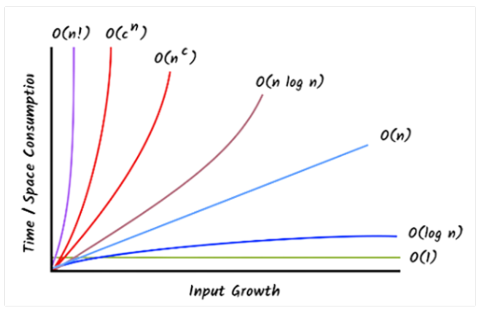
The computational complexity analysis of algorithms is a measure of its efficiency in terms of resources required. It has an effect on speed and performance, with lesser complexity indicating faster execution and higher complexity signifying failure or bad performance. Linear, exponential, logarithmic, quadratic, cubic, or constant complexity are possible, with quicker algorithms having more favorable complexities.

What is complexity analysis in data structure and algorithms?

Complexity analysis is a method for describing how long an algorithm takes depending on the size of the input (independent of the machine, language, and compiler). It is utilized to assess how different algorithms' execution times vary.

What is the need for Complexity Analysis?

  • Execution time and space requirements are determined through complexity analysis.
  • It is used to compare different algorithms with varying input sizes.
  • The complexity of a problem aids in determining its difficulty.
  • A problem's difficulty can often be determined by the amount of time and memory (memory) required to solve it.

Asymptotic Notations in Complexity Analysis

Big O Notation

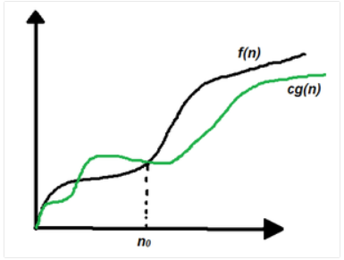
  • Big-O notation is used to express an algorithm's maximum permissible running time.
  • As a result, it provides an algorithm's worst-case complexity.
  • We can asymptotically limit the extension of a running time to a range of constant factors above and below by utilizing a large O-notation.
  • It is a model for measuring the effectiveness of algorithms. 

Omega Notation

  • The lowest bound of an algorithm's running time is shown in omega notation.
  • As a result, it offers an algorithm's best-case complexity.
  • The execution time acts as a lower bound on the time complexity of the algorithm.
  • It is described as the circumstance under which an algorithm can execute a statement in the quickest possible time.

Theta Notation

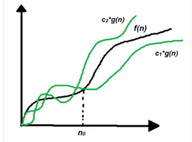
  • The function is enclosed in the theta notation from above and below.
  • It is used to examine the average-case complexity of an algorithm because it represents the upper and lower bounds of the running time of an algorithm.
  • The execution time acts as a lower and upper bound on the time complexity of the algorithm.
  • It is present as both the greatest and smallest bounds for a certain input value.

Little ο asymptotic notation

  • Although, as written, Big- can also be a loose upper bound, it is used as a tight upper bound on the growth of an algorithm's effort (this effort is described by the function f(n)).
  • A tight upper bound is referred to as having a “Little-o” (ο()) notation. 

Little ω asymptotic notation

  • Allow the functions f(n) and g(n) to map positive integers to positive real numbers.
  • We say that f(n) is ω(g(n)) (or f(n) ∈ ω(g(n))) if for any genuine constant c > 0, the existence of an integer constant n0 ≥ 1 such that f(n) > c * g(n) ≥ 0 for every integer n ≥ n0. 

Types of Complexities 

Time Complexity

When compared to the size of its input, an algorithm's time complexity indicates how long it will take to complete. As a function of the input size, it gives an upper bound on the running time. Measuring is frequently written using Big O notation, which specifies the maximum growth rate relative to the input size (e.g., O(n), O(log n), O(n2), etc.).

Example

def find_max(arr):    max_element = arr[0]
    for element in arr:
        if element > max_element:
            max_element = element
    return max_element

Explanation

Due to the algorithm's single loop of the array and the fact that the number of iterations varies linearly on the input array's size, the time complexity in this example is O(n).

Space Complexity

The amount of memory that an algorithm requires in relation to the size of the input is measured as space complexity. It contains both input space (memory needed to store the input) and auxiliary space (memory utilized by the method itself). It is frequently represented using Big O notation, just like time complexity, to describe the maximum allowable amount of memory utilization.

Example

def fibonacci(n):    if n <= 1:
        return n
    else:
        return fibonacci(n-1) + fibonacci(n-2)

Explanation

The procedure in this example uses a recursive stack that increases linearly with the input value n, hence the space complexity is O(n).

Auxiliary Space Complexity

Auxiliary space complexity is a measure of how much space an algorithm uses in addition to its input and any primary data structures. Input space is not included. It also expresses the upper bound of additional memory used and uses Big O notation.

Example

def reverse_array(arr):    start = 0
    end = len(arr) - 1
    while start < end:
        arr[start], arr[end] = arr[end], arr[start]
        start += 1
        end -= 1

Explanation

The procedure utilizes a fixed amount of extra space regardless of the size of the input, hence, in this case, the auxiliary space complexity is O(1). Without using more memory, it switches elements while they are still in place.

How does Complexity affect any algorithm?

  • The amount of time an algorithm requires to run as a function of the length of the input is measured by its temporal complexity.  
  • The algorithm's space complexity estimates how much memory or storage it needs to operate as a function of the size of the input.

How to optimize the time and space complexity of an Algorithm?

Optimizing entails changing a problem's brute-force solution. In order to solve the problem in the shortest amount of time and with the least amount of complexity, the best solution is determined. A program can be made more efficient by either limiting the search space at each stage or using less space right away. Both time and space optimization can be used to improve a solution. A program can be improved by:

  • By implementing appropriate algorithms, we can reduce both time and space complexity.
  • We can reduce the time required to run the program and increase the space occupied.
  • We can reduce the memory consumption of the program and increase its overall run duration.

Different types of Complexity exist in the program

Constant Complexity

If the program's function or method requires very little time to execute. It will then be regarded as constant complexity. 

Example

Python

def constant_time_operation(data):

    # This operation takes a fixed amount of time (O(1)) because it doesn't depend on the input size.

    return data[0]

# Example usage:

my_list = [1, 2, 3, 4, 5]

result = constant_time_operation(my_list)

print(result)

Java

public class ConstantTimeOperation {

    public static int constantTimeOperation(int[] data) {

        // This operation takes a fixed amount of time (O(1)) because it doesn't depend on the input size.

        return data[0];

    }

    public static void main(String[] args) {

        int[] myArray = {1, 2, 3, 4, 5};

        int result = constantTimeOperation(myArray);

        System.out.println(result);

    }

}

C++

#include <iostream>

class ConstantTimeOperation {

public:

    static int constantTimeOperation(int data[]) {

        // This operation takes a fixed amount of time (O(1)) because it doesn't depend on the input size.

        return data[0];

    }

};

int main() {

    int myArray[] = {1, 2, 3, 4, 5};

    int result = ConstantTimeOperation::constantTimeOperation(myArray);

    std::cout << result << std::endl;

    return 0;

}

Explanation

In order to retrieve and print the first element of an array, this example defines a class with a static method that retrieves the first element of an integer array.

Output

1

Logarithmic Complexity

It has an O(log(N) complexity requirement. It goes through the process of doing the order of log(N) steps. It frequently uses logarithmic base 2 to execute operations on N elements. 

Example

Python

def binary_search(arr, target):

    left, right = 0, len(arr) - 1

    while left <= right:

        mid = (left + right) // 2

        if arr[mid] == target:

            return mid # Found the target element

        elif arr[mid] < target:

            left = mid + 1

        else:

            right = mid - 1

    return -1 # Target element not found

# Example usage:

arr = [1, 2, 3, 4, 5, 6, 7, 8, 9, 10]

target = 6

result = binary_search(arr, target)

if result != -1:

    print(f"Element {target} found at index {result}")

else:

    print(f"Element {target} not found in the array")

Java

public class BinarySearch {

    public static int binarySearch(int[] arr, int target) {

        int left = 0;

        int right = arr.length - 1;

        while (left <= right) {

            int mid = left + (right - left) / 2;

            if (arr[mid] == target) {

                return mid; // Found the target element

            } else if (arr[mid] < target) {

                left = mid + 1;

            } else {

                right = mid - 1;

            }

        }

        return -1; // Target element not found

    }

    public static void main(String[] args) {

        int[] arr = {1, 2, 3, 4, 5, 6, 7, 8, 9, 10};

        int target = 6;

        int result = binarySearch(arr, target);

        if (result != -1) {

            System.out.println("Element " + target + " found at index " + result);

        } else {

            System.out.println("Element " + target + " not found in the array");

        }

    }

}

C++

#include <iostream>

#include <vector>

class BinarySearch {

public:

    static int binarySearch(std::vector<int>& arr, int target) {

        int left = 0;

        int right = arr.size() - 1;

        while (left <= right) {

            int mid = left + (right - left) / 2;

            if (arr[mid] == target) {

                return mid; // Found the target element

            } else if (arr[mid] < target) {

                left = mid + 1;

            } else {

                right = mid - 1;

            }

        }

        return -1; // Target element not found

    }

};

int main() {

    std::vector<int> arr = {1, 2, 3, 4, 5, 6, 7, 8, 9, 10};

    int target = 6;

    int result = BinarySearch::binarySearch(arr, target);

    if (result != -1) {

        std::cout << "Element " << target << " found at index " << result << std::endl;

    } else {

        std::cout << "Element " << target << " not found in the array" << std::endl;

    }

    return 0;

}

Explanation

In the provided example, a binary search is used to locate the target element (in this case, 6), which is located within the sorted array arr. 

Output

Element 6 found at index 5

Linear Complexity

It imposes an O(N) complexity. It includes exactly as many steps as there are elements in total to carry out an operation on N elements.

Example

Python

def linear_sum(arr):

    total = 0

    for num in arr:

        total += num

    return total

# Example usage:

my_list = [1, 2, 3, 4, 5]

result = linear_sum(my_list)

print("Sum of elements:", result)

Java

public class LinearSum {

    public static int linearSum(int[] arr) {

        int total = 0;

        for (int num : arr) {

            total += num;

        }

        return total;

    }

    public static void main(String[] args) {

        int[] myArray = {1, 2, 3, 4, 5};

        int result = linearSum(myArray);

        System.out.println("Sum of elements: " + result);

    }

}

C++

#include <iostream>

int linearSum(int arr[], int size) {

    int total = 0;

    for (int i = 0; i < size; ++i) {

        total += arr[i];

    }

    return total;

}

int main() {

    int myArray[] = {1, 2, 3, 4, 5};

    int size = sizeof(myArray) / sizeof(myArray[0]);

    int result = linearSum(myArray, size);

    std::cout << "Sum of elements: " << result << std::endl;

    return 0;

}

Explanation

This example computes the array's myArray's element sum and prints the result. 

Output

Sum of elements: 15

Quadratic Complexity

It requires an O(n2) level of complexity. In order to solve a given problem, it performs the order of N2 count of operations on N number of items for N input data size.

Example

Python

def find_pairs_with_sum(arr, target_sum):

    pairs = []

    n = len(arr)

    for i in range(n):

        for j in range(i + 1, n):

            if arr[i] + arr[j] == target_sum:

                pairs.append((arr[i], arr[j]))

    return pairs

# Example usage

arr = [1, 2, 3, 4, 5]

target_sum = 7

result = find_pairs_with_sum(arr, target_sum)

print(result) # Output: [(2, 5), (3, 4)]

Java

import java.util.ArrayList;

import java.util.List;

public class FindPairsWithSum {

    public static List<int[]> findPairsWithSum(int[] arr, int targetSum) {

        List<int[]> pairs = new ArrayList<>();

        int n = arr.length;

        for (int i = 0; i < n; i++) {

            for (int j = i + 1; j < n; j++) {

                if (arr[i] + arr[j] == targetSum) {

                    pairs.add(new int[]{arr[i], arr[j]});

                }

            }

        }

        return pairs;

    }

    public static void main(String[] args) {

        int[] arr = {1, 2, 3, 4, 5};

        int targetSum = 7;

        List<int[]> result = findPairsWithSum(arr, targetSum);

        for (int[] pair : result) {

            System.out.println("(" + pair[0] + ", " + pair[1] + ")");

        }

    }

}

C++

#include <iostream>

#include <vector>

std::vector<std::pair<int, int>> findPairsWithSum(int arr[], int size, int targetSum) {

    std::vector<std::pair<int, int>> pairs;

    for (int i = 0; i < size; i++) {

        for (int j = i + 1; j < size; j++) {

            if (arr[i] + arr[j] == targetSum) {

                pairs.push_back(std::make_pair(arr[i], arr[j]));

            }

        }

    }

    return pairs;

}

int main() {

    int arr[] = {1, 2, 3, 4, 5};

    int targetSum = 7;

    int size = sizeof(arr) / sizeof(arr[0]);

    std::vector<std::pair<int, int>> result = findPairsWithSum(arr, size, targetSum);

    for (const std::pair<int, int>& pair : result) {

        std::cout << "(" << pair.first << ", " << pair.second << ")" << std::endl;

    }

    return 0;

}

Explanation

The example searches the arr list for pairs of elements whose sum equals the target_sum, then outputs the finding.

Output

[(2, 5), (3, 4)]

Factorial Complexity

For N input data size, it executes the order of N! steps on N elements to solve a given problem, imposing a complexity of O(n!).

Example

Python

def factorial(n):

    if n == 0:

        return 1

    else:

        return n * factorial(n - 1)

# Example usage:

number = 5

result = factorial(number)

print(f"The factorial of {number} is {result}")

Java

public class Factorial {

    public static int factorial(int n) {

        if (n == 0) {

            return 1;

        } else {

            return n * factorial(n - 1);

        }

    }

    public static void main(String[] args) {

        int number = 5;

        int result = factorial(number);

        System.out.println("The factorial of " + number + " is " + result);

    }

}

C++

#include <iostream>

int factorial(int n) {

    if (n == 0) {

        return 1;

    } else {

        return n * factorial(n - 1);

    }

}

int main() {

    int number = 5;

    int result = factorial(number);

    std::cout << "The factorial of " << number << " is " << result << std::endl;

    return 0;

}

Explanation

This example shows a typical recursive programming pattern by computing the factorial of a number (in this case, 5), using a recursive function, and printing the result.

Output

The factorial of 5 is 120

Exponential Complexity

It imposes complexity in the order of O(2N), O(N!), and O(nk). It will carry out the operations in a count that is exponentially dependent on the size of the input data for N elements. 

Example

Python

def fibonacci_memoization(n, memo={}):

    if n in memo:

        return memo[n]

    if n <= 1:

        return n

    else:

        result = fibonacci_memoization(n - 1, memo) + fibonacci_memoization(n - 2, memo)

        memo[n] = result

        return result

n = 100 # Change this to the desired Fibonacci number

result = fibonacci_memoization(n)

print(f"The {n}-th Fibonacci number is {result}")

Java

import java.util.HashMap;

import java.util.Map;

public class FibonacciMemoization {

    private static Map<Integer, Long> memo = new HashMap<>();

    public static long fibonacciMemoization(int n) {

        if (memo.containsKey(n)) {

            return memo.get(n);

        }

        if (n <= 1) {

            return n;

        } else {

            long result = fibonacciMemoization(n - 1) + fibonacciMemoization(n - 2);

            memo.put(n, result);

            return result;

        }

    }

    public static void main(String[] args) {

        int n = 100; // Change this to the desired Fibonacci number

        long result = fibonacciMemoization(n);

        System.out.printf("The %d-th Fibonacci number is %d%n", n, result);

    }

}

C++

#include <iostream>

#include <unordered_map>

std::unordered_map<int, long long> memo;

long long fibonacciMemoization(int n) {

    if (memo.find(n) != memo.end()) {

        return memo[n];

    }

    if (n <= 1) {

        return n;

    } else {

        long long result = fibonacciMemoization(n - 1) + fibonacciMemoization(n - 2);

        memo[n] = result;

        return result;

    }

}

int main() {

    int n = 100; // Change this to the desired Fibonacci number

    long long result = fibonacciMemoization(n);

    std::cout << "The " << n << "-th Fibonacci number is " << result << std::endl;

    return 0;

}

Explanation

This example efficiently calculates the n-th Fibonacci number using memoization. To avoid repeating operations, previously computed Fibonacci numbers are kept in a dictionary (memo), and the result is then printed for n = 100.

Output

The 100-th Fibonacci number is 354224848179261915075

Worst Case time complexity of different data structures for different operations

Data structureAccessSearchInsertionDeletion
ArrayO(1)O(N)O(N)O(N)
StackO(N)O(N) O(1) O(1)
QueueO(N)O(N) O(1) O(1)
Singly Linked ListO(N)O(N)O(N)O(N)
Doubly Linked ListO(N)O(N) O(1) O(1)
Hash TableO(N)O(N)O(N)O(N)
Binary Search TreeO(N)O(N)O(N)O(N)
AVL TreeO(log N)O(log N)O(log N)O(log N)
Binary TreeO(N)O(N)O(N)O(N)
Red Black TreeO(log N)O(log N)O(log N)O(log N)

FAQs

1. What are the two types of complexity analysis in data structure and algorithms?

Time complexity and space complexity are the two categories of complexity analysis.

2. What are the 4 categories of complexity?

Time complexity, space complexity, computational complexity, and algorithmic complexity are the four types of complexity.

3. What are the different forms of complexity?

Algorithmic complexity, structural complexity, and behavioral complexity are a few examples of complexity.

4. How do you find the complexity of an algorithm in data structure?

Analyze the number of basic operations and memory usage as a function of input size to determine the time and space complexity of an algorithm in a data structure.

Summary

What currency is to every individual to sustain, so are algorithmic analysis and complexities to a programmer. The programmer uses the outcome of the algorithmic analysis as a guideline for program development, and the complexities prevent him from the incorrect choices in designing a solution to the program. The time complexity of the algorithm is an estimation of how much time or space an algorithm will require to process a given volume of data.

Share
About Author
Shailendra Chauhan (Microsoft MVP, Founder & CEO at DotNetTricks)

Shailendra Chauhan is the Founder and CEO at ScholarHat by DotNetTricks which is a brand when it comes to e-Learning. He provides training and consultation over an array of technologies like Cloud, .NET, Angular, React, Node, Microservices, Containers and Mobile Apps development. He has been awarded Microsoft MVP 8th time in a row (2016-2023). He has changed many lives with his writings and unique training programs. He has a number of most sought-after books to his name which has helped job aspirants in cracking tough interviews with ease.
Accept cookies & close this