


18
JunData Structure Cheat Sheet: Complete Guide
23 Sep 2025
Career
5.61K Views
37 min read

Learn with an interactive course and practical hands-on labs
Free DSA Online Course with Certification
The data structure cheat sheet is a comprehensive guide for beginners and intermediate learners who want to master the core concepts of data structures used in programming and system design.
This data structure cheat sheet covers everything from basic arrays and linked lists to advanced structures like trees, heaps, graphs, and tries. With simple definitions, time complexities, code snippets, and use cases, this guide will also help you to understand how data is stored, accessed, and managed efficiently. 90% of developers land jobs faster with DSA mastery – Join our Free Data Structure and Algorithm Course and get certified.
Whether you are preparing for coding interviews or working on real-world applications, this cheat sheet provides a quick and practical reference for all essential data structures, So Let's Start.
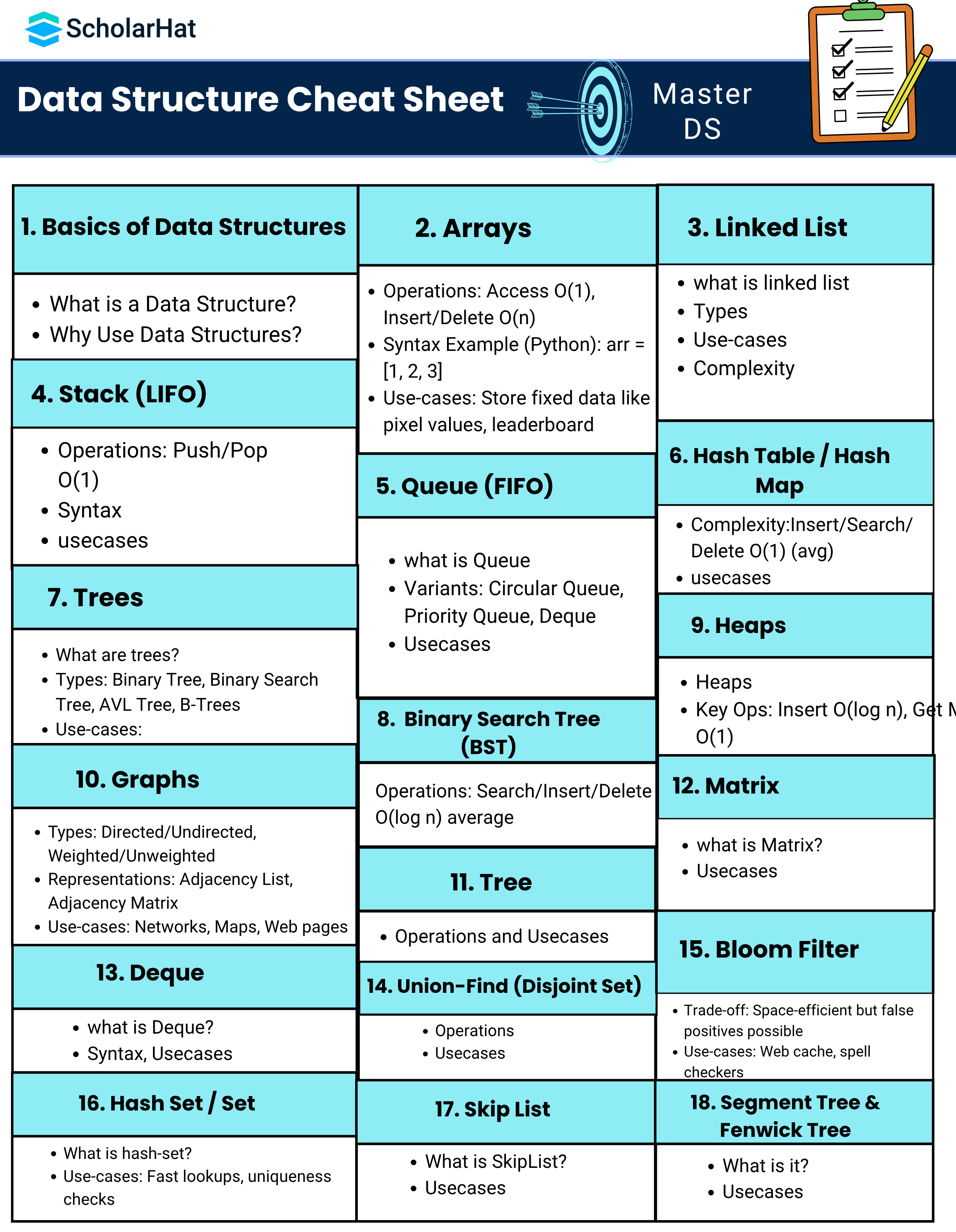
Step 1: Basics of Data Structures
What is a Data Structure?
A data structure is a specialized format or technique used to organize, process, retrieve, and store data efficiently. It is a fundamental concept in computer science that enables optimal performance for operations such as searching, sorting, inserting, deleting, and traversing data.
“A data structure is a way of organizing and storing data so that it can be accessed and worked with effectively.”
- Real-Life Analogy: Think of a bookshelf as a data structure. It helps organize books (data) in a specific way by genre, author, or title so you can find and retrieve a book quickly when needed.
Classification of Data Structures
Data structures are primarily classified into two categories:
1. Linear Data Structures:
- Elements are arranged in a sequential order.
- Each element is connected to its previous and next element (except the first and last).
- Examples: Array, Linked List, Stack, Queue
2. Non-Linear Data Structures:
- In non-linear data structures elements are not arranged sequentially.
- They are connected in hierarchical or graph-like structures.
- Examples: Tree, Graph, Hash Table (partially)
| Type | Description | Example Use Case |
| Linear | Stores data in a single level or line | Browsing history using a stack |
| Non-Linear | Stores data in branching formats | File systems using trees |
Why Use Data Structures?
Using appropriate data structures is crucial for writing efficient programs and solving complex problems. Here's why:
1. Efficient Data Management
- Data structures help in organizing data so it can be accessed, processed, and modified easily.
- Example: Arrays store elements at contiguous memory locations, allowing fast access by index.
2. Improved Algorithm Performance
- Choosing the right data structure improves time and space complexity.
- Example: Hash tables provide O(1) average-time complexity for lookups, compared to O(n) in linear searches.
3. Optimized Memory Usage
- Structures like linked lists allocate memory dynamically to avoid wastage.
- Example: Unlike arrays, linked lists don’t require predefined sizes and grow as needed.
Real-World Use Cases
| Scenario | Data Structure Used | Why? |
| Navigating browser history | Stack | Follows LIFO (Last-In-First-Out) |
| Task scheduling | Queue | Follows FIFO (First-In-First-Out) |
| Social network connections | Graph | Represents relationships between users |
| Searching a file system | Tree | Represents folder hierarchy |
Key Takeaways
- Data structures are essential for organizing and managing data efficiently.
- They are broadly classified as Linear (e.g., arrays, stacks) and Non-Linear (e.g., trees, graphs).
- They enhance algorithm performance, enable faster data access, and help with memory optimization.
- Mastering data structures is foundational for every programmer and developer.
Step 2: Arrays
What is an Array?
An array is a fixed-size, sequential collection of same-type elements stored in contiguous memory locations. It allows random access and is best for storing and retrieving uniform data types efficiently.
Memory Representation
Elements are stored side by side in memory. This allows fast access but makes inserting or deleting from the middle more expensive.
Index:     0     1     2     3
Array:   [10]  [20]  [30]  [40]
Key Characteristics of Arrays
- Fixed Size: The size of the array is defined at creation.
- Same Data Type: All elements are of the same type.
- Contiguous Memory: Data is stored in adjacent memory blocks.
- Random Access: Direct access to any element using its index.
| Read More: Types of Arrays in Data Structures |
Syntax Examples
Python
arr = [1, 2, 3]
print(arr[0])  # Output: 1
C
int arr[3] = {1, 2, 3};
printf("%d", arr[0]); // Output: 1
Java
int[] arr = {1, 2, 3};
System.out.println(arr[0]); // Output: 1
Common Operations on Arrays
| Operation | Description | Time Complexity |
| Access | Get element at a given index | O(1) |
| Update | Set element at a specific index | O(1) |
| Insert (middle) | Insert a new element with shifting | O(n) |
| Delete (middle) | Remove element and shift remaining elements | O(n) |
| Traverse | Visit each element | O(n) |
Types of Arrays
1. One-Dimensional Array
It is a simple linear array that holds data in a single row.
marks = [90, 85, 70, 60]
Use case: Store values like marks, temperatures, salaries.
2. Two-Dimensional Array
It is also known as a matrix. Stores data in rows and columns like a table.
matrix = [
  [1, 2, 3],
  [4, 5, 6],
  [7, 8, 9]
]
Use case: Grids, game boards, image pixels.
3. Multi-Dimensional Array
These are the arrays with more than two dimensions. Arrays within arrays.
cube = [
  [[1, 2], [3, 4]],
  [[5, 6], [7, 8]]
]
Use case: 3D modeling, simulations.
4. Dynamic Array
Arrays that can grow or shrink during runtime.
arr = [1, 2, 3]
arr.append(4)
Use case: Storing user input or runtime data.
5. Jagged Array
Array of arrays where each sub-array can have a different length.
jagged = [
  [1, 2, 3],
  [4, 5],
  [6]
]
Use case: Variable subject marks, triangle patterns.
Key Takeaways
- Arrays are used for storing fixed-size, same-type data sequentially
- They offer fast access (O(1)) but slow insertion and deletion (O(n))
- There are different types of arrays suited for various applications
- Arrays are fundamental for more complex data structures like matrices and heaps
Step 3: Linked List
What is a Linked List?
A linked list is a linear data structure in which elements called nodes are not stored in contiguous memory. Each node contains two parts:
- Data - the actual value
- Pointer - a reference to the next node in the sequence
Unlike arrays, linked lists are dynamic in nature and grow or shrink as needed, making memory usage efficient for certain operations.
Real-Life Analogy
Imagine a treasure map where each location has:
- A clue representing the data
- A direction to the next clue representing the pointer
You must follow the map step-by-step, just like traversing a linked list from head to tail.
Characteristics of Linked List
- Dynamic size
- Non-contiguous memory allocation
- Sequential access only
- Efficient insert and delete at head
Syntax Example in Python
class Node:
def __init__(self, data):
self.data = data
self.next = None
node1 = Node(10)
node2 = Node(20)
node1.next = node2
Types of Linked Lists
1. Singly Linked List
Each node points to the next node. Traversal is one-way from head to tail.
Head -> 10 -> 20 -> 30 -> None
2. Doubly Linked List
Each node has two pointers: next and previous. Traversal can be both forward and backward.
None <- 10 <-> 20 <-> 30 -> None
3. Circular Linked List
Last node points back to the first node. Can be singly or doubly linked.
10 -> 20 -> 30 -> points back to 10
Key Takeaways
- Linked list is a dynamic, flexible data structure made of nodes
- Each node contains data and a pointer to the next node
- Types include singly, doubly, and circular linked lists
- Efficient for insertion and deletion but slower for direct access
- Ideal for applications with frequent additions or deletions
Step 4: Stack
What is a Stack?
A stack is a linear data structure that follows the Last In First Out principle. This means the last element added to the stack is the first one to be removed.
Real Life Analogy
Imagine a stack of plates in your kitchen:
- You place a new plate on top of the stack
- You remove the topmost plate first
This is how a stack works in programming. The most recent item added is the first one removed.
Characteristics of a Stack
- LIFO Order Last In First Out
- Restricted Access Only the top element can be accessed
- Two Main Operations:
- Push Add an element to the top
- Pop Remove the top element
Python Syntax Example
stack = []
stack.append(10)
stack.append(20)
top = stack.pop()  # Returns 20
Stack Operations and Time Complexity
| Operation | Description | Time Complexity |
| Push | Add element to the top | O(1) |
| Pop | Remove top element | O(1) |
| Peek | View top element without removing | O(1) |
| isEmpty | Check if the stack is empty | O(1) |
| Size | Count number of elements | O(1) |
Stack Working Example
Initial Stack: []
Push 10       → [10]
Push 20       → [10, 20]
Pop           → [10]  (Removed 20)
Stack Implementation Options
- Array or List Based Stack using Python list or Java array
- Linked List Based Stack where each node points to the next
- Built in Libraries:
- Python collections.deque or queue.LifoQueue
- Java java.util.Stack
Key Takeaways
- A stack uses the LIFO principle and is ideal for tracking recent actions
- Push and pop operations are performed in constant time O1
- Used in undo features, function calls, expression parsing, and more
- Simple to implement using arrays, linked lists, or built in libraries
Step 5: Queue
What is a Queue?
A queue is a linear data structure that follows the First In First Out principle. The element inserted first is removed first, just like standing in a real life line.
Real Life Analogy
Imagine a queue of people at a ticket counter:
- The first person to enter the queue is the first to get the ticket and leave
- New people join at the end, and service happens from the front
Characteristics of a Queue
- FIFO Order First In First Out
- Two Ends:
- Front for removing elements dequeue
- Rear for inserting elements enqueue
- No random access of elements
Python Syntax Example
from collections import deque
queue = deque()
queue.append(10)
queue.append(20)
front = queue.popleft()  # Returns 10
Queue Operations and Time Complexity
| Operation | Description | Time Complexity |
| Enqueue | Add element at rear | O(1) |
| Dequeue | Remove element from front | O(1) |
| Peek | View front element | O(1) |
| isEmpty | Check if queue is empty | O(1) |
| Size | Count number of elements | O(1) |
Queue Working Example
Initial Queue: []
Enqueue 10    → [10]
Enqueue 20    → [10, 20]
Dequeue       → [20]  Removed 10
Types of Queues
1. Simple Queue
- Basic FIFO structure. Insert at rear and remove from front.
2. Circular Queue
- The last position connects back to the first, forming a circle. Efficient use of memory in fixed size arrays.
3. Priority Queue
- Each element has a priority. Elements are dequeued based on priority, not arrival time.
4. Double Ended Queue Deque
- Insertion and deletion can happen from both ends. Python collections.deque supports this.
Key Takeaways
- A queue follows the FIFO principle and is ideal for fair processing of tasks
- Main operations are enqueue and dequeue, both performed in constant time
- Queues come in various forms like circular queue, priority queue, and deque
- Widely used in task scheduling, resource management, and graph algorithms
Step 6: Hash Table or Dictionary
- Definition: Maps keys to values using a hash function.
- Complexity: Insert Search Delete O1 average case
- Use cases: Caching, symbol tables, fast lookup
Time Complexity Average O 1 for Insert Search and Delete
data = dict
data apple = 3
data banana = 5
print data apple
Step 7: Tree
What is a Tree?
A Tree is a non linear hierarchical data structure that consists of nodes connected by edges. It starts with a root node at the top. Each node can have zero or more child nodes. Unlike graphs, there are no cycles in trees.
Real Life Analogy
Think of a family tree. You are connected to your parents and children in a hierarchical manner. The root could be your grandparents, branching down to you and your siblings.
Characteristics of Trees
- One node is always the root
- Every node has one parent except root
- Nodes may have zero or more children
- No cycles only one path between any two nodes
Basic Terminology
| Term | Description |
|---|---|
| Root | Topmost node |
| Parent | Node that points to child nodes |
| Child | Node that descends from a parent |
| Leaf | Node with no children |
| Subtree | A child node and all its descendants |
| Depth | Number of edges from root to the node |
| Height | Number of edges from node to the deepest leaf |
| Edge | Connection between one node and another |
Syntax Example Python
class Node:
    def __init__(self, data):
        self.data = data
        self.left = None
        self.right = None

# Creating a simple tree
root = Node(10)
root.left = Node(5)
root.right = Node(15)
Types of Trees
- Binary Tree Each node has at most 2 children left and right
- Binary Search Tree BST Left child is smaller right child is greater than the parent node
- Balanced Tree Height difference between left and right subtrees is minimal
- AVL Tree Self balancing BST where the balance factor is maintained
- Heap A complete binary tree used in priority queues
- N ary Tree A node can have more than two children
Tree Traversals
| Type | Description |
|---|---|
| Inorder | Left Subtree Root Right Subtree |
| Preorder | Root Left Subtree Right Subtree |
| Postorder | Left Subtree Right Subtree Root |
| Level Order | Traverse level by level uses a queue |
Key Takeaways
- A tree is a hierarchical data structure with a root children and no cycles
- Common operations include insertion deletion traversal and search
- Binary trees and their variants like BST AVL Heaps are widely used
- Trees are essential in searching organizing and hierarchical data modeling
Step 8: Binary Search Tree (BST)
A Binary Search Tree (BST) is a special type of binary tree where each node follows this rule:
- The left child contains a value less than its parent node.
- The right child contains a value greater than its parent node.
Key Operations
- Search: Starting from the root, recursively move left or right depending on whether the value is smaller or greater than the current node.
- Insert: Follows the same logic as search—traverse the tree and place the new value at the appropriate leaf position.
- Delete: Three cases:
- Node is a leaf (no children): simply remove it.
- Node has one child: link the child directly to the parent.
- Node has two children: replace with the in-order successor (smallest in the right subtree) or predecessor.
Time Complexity
- Average case: O(log n)
- Worst case: O(n) – occurs in skewed trees (like linked lists)
Important Note
A BST can become unbalanced (skewed) if data is inserted in a sorted manner. This causes all elements to fall to one side (left or right), degrading performance to linear time. To avoid this, we use self-balancing trees like AVL Trees or Red-Black Trees.
Use-Cases
- Autocomplete or Auto-suggestion systems
- Efficient range queries (like finding values within a range)
- Maintaining sorted data in real-time
- Dictionary/map implementations
BST Insertion Example in C
// Define a node
struct Node {
    int data;
    struct Node* left;
    struct Node* right;
};

// Create a new node
struct Node* createNode(int value) {
    struct Node* newNode = (struct Node*)malloc(sizeof(struct Node));
    newNode->data = value;
    newNode->left = newNode->right = NULL;
    return newNode;
}

// Insert into BST
struct Node* insert(struct Node* root, int value) {
    if (root == NULL) return createNode(value);

    if (value < root->data)
        root->left = insert(root->left, value);
    else if (value > root->data)
        root->right = insert(root->right, value);

    return root;
}

// Inorder traversal (prints in sorted order)
void inorder(struct Node* root) {
    if (root != NULL) {
        inorder(root->left);
        printf("%d ", root->data);
        inorder(root->right);
    }
}
Real-World Example
Imagine an online store with product IDs. A BST can be used to store and manage these IDs so that:
- Searching for a specific product is fast (O(log n))
- Inserting new products keeps the list sorted automatically
- You can easily display products within a certain ID range
Step 9: Heaps
A heap is a special complete binary tree that maintains the heap property. It is widely used when quick access to the smallest or largest element is required.
There are two main types of heaps:
- Min Heap - The smallest element is always at the root.
- Max Heap - The largest element is always at the root.
Heaps are usually implemented as arrays where:
- Left child of index i is at 2i + 1
- Right child of index i is at 2i + 2
- Parent of index i is at floor of (i - 1) / 2
- Time Complexity: Insert and Delete take Olog n time, Get Min or Max takes O1.
- Use cases: Priority queues, CPU scheduling, Dijkstras algorithm, sorting k lists, memory management.
Python Program Example:
import heapq
min_heap = []
heapq.heappush(min_heap, 10)
heapq.heappush(min_heap, 5)
heapq.heappush(min_heap, 15)

print("Minimum element:", min_heap[0])  # Output: 5

heapq.heappop(min_heap)
print("Heap after pop:", min_heap)  # Output: [10, 15]
This program demonstrates a min heap using Python's built-in heapq module.
Step 10: Graphs
- Definition A set of nodes connected by edges used to model networks
- Types Directed Undirected Weighted
- Represented using Adjacency Matrix or Adjacency List
- Use Case GPS Routing Social Networks Web Crawling
Step 11: Tries
- Definition: Tree like data structure for string storage
- Use Case Auto complete Spell checker Word Dictionary
- Time Complexity O L where L is length of word
Step 12: Matrix
Definition: A matrix is a collection of elements arranged in a two-dimensional grid. Each element is accessed using two indices: row and column.
Syntax (in C-like pseudocode):
int matrix[3][3] = {
  {1, 2, 3},
  {4, 5, 6},
  {7, 8, 9}
};
Key Operations:
- Access: matrix[i][j]
- Traversal: Nested loops
- Transpose, Rotate
- Matrix Multiplication
Use Cases:
- Image processing
- Graph representation (adjacency matrix)
- 2D games (e.g., chessboard)
- Mathematical computation
Step 13: Deque (Double-Ended Queue)
Definition: Unlike a queue or stack, a deque can operate at both front and rear ends.
Key Operations:
- push_front(), push_back()
- pop_front(), pop_back()
- front(), back()
- Check if empty, get size
Use Cases:
- Browser history navigation
- Sliding window problems
- Palindrome checker
- Task scheduling
Example (Python deque):
from collections import deque
d = deque()
d.append(1)
d.appendleft(2)
print(d)  # Output: deque([2, 1])
Step 14: Union-Find (Disjoint Set)
Definition: Used to keep track of elements which are split into one or more disjoint sets. Key operations are Find and Union.
Key Operations:
- find(x): Find the root of x
- union(x, y): Merge the sets containing x and y
- Optimizations: Path compression, Union by rank
Use Cases:
- Detecting cycles in graphs
- Kruskal’s MST algorithm
- Network connectivity
- Social network friend groups
Example (Python-style):
parent = [i for i in range(n)]

def find(x):
    if parent[x] != x:
        parent[x] = find(parent[x])
    return parent[x]

def union(x, y):
    parent[find(x)] = find(y)
Step 15: Bloom Filter
Definition: It allows for false positives (may say "yes" when it's "no") but never false negatives. It uses multiple hash functions.
Key Operations:
- add(item)
- might_contain(item)
Use Cases:
- Spell checkers
- Web cache filtering
- Email spam detection
- Database query optimization
Advantages:
- Space-efficient
- Fast insert and lookup
Limitation:
- No deletion
- False positives possible
Step 16: HashSet
Definition: It stores elements in a hash table and provides average O(1) time complexity for add, remove, and lookup operations.
Key Operations:
- add(x)
- remove(x)
- contains(x)
Use Cases:
- Removing duplicates
- Checking existence
- Set operations (union, intersection)
Example (Java):
HashSet<String> set = new HashSet<>();
set.add("apple");
set.add("banana");
System.out.println(set.contains("apple")); // true
Step 17: Skip List
Definition: It's a layered linked list where each higher level acts as an "express lane" over the list, reducing the time complexity.
Key Operations:
- Insert: O(log n)
- Delete: O(log n)
- Search: O(log n)
Use Cases:
- Databases (Redis, LevelDB)
- In-memory key-value stores
- Ordered maps or sets
Structure: Each node can have multiple forward pointers. Levels are chosen randomly to balance the structure.
Step 18: Segment Tree
Definition: Each node represents an interval and stores a summary (like sum, min, or max) of that interval.
Key Operations:
- build() – O(n)
- query(l, r) – O(log n)
- update(index, value) – O(log n)
Use Cases:
- Range sum/min/max queries
- Lazy propagation (for range updates)
- Competitive programming
- Interval problems
Example Use Case:
Array = [2, 4, 5, 7, 8]
Query: sum(1, 3) → output = 4 + 5 + 7 = 16
Conclusion
Understanding data structures is the foundation of writing efficient and scalable code. From basic arrays to advanced trees and graphs, each data structure serves a specific purpose and comes with its own strengths and weaknesses. Choosing the right data structure can drastically improve the performance of your programs in terms of time and memory usage.
Only 2% of Java Developers become Solution Architects. Don’t get left behind—Enroll now in our Java Architect Certification and secure your career growth & 60% higher salary potential.
FAQs
- Data Structure is a way to store and organize data.
- Algorithm is a step-by-step procedure to perform a specific task using data structures.
The four basic data structure types are linear data structures, tree data structures, hash data structures and graph data structures
- Arrays
- Linked Lists
- Stacks
- Queues
- Trees
- Graphs
- Hash Tables
- Heaps
Take our Datastructures skill challenge to evaluate yourself!

In less than 5 minutes, with our skill challenge, you can identify your knowledge gaps and strengths in a given skill.