Quick Sort Algorithm in Data Structures - Its Types ( With Examples )

Quick Sort algorithm is a highly efficient sorting technique used to arrange data in ascending or descending order. The Quick Sort algorithm works by selecting a pivot element and partitioning the array around it, sorting smaller parts recursively. One of the key reasons the Quick Sort algorithm is important is because of its fast performance, with an average-case time complexity of O(n log n). It is widely used in programming, especially when dealing with large datasets.

In this DSA tutorial, we will explore the Quick Sort algorithm, understand how it works, and learn why it is one of the most efficient sorting techniques used in real-world applications.

What is Quick Sort in Data Structures?

Quick sort is a highly efficient, comparison-based sorting algorithm that follows the divide-and-conquer strategy. It works by selecting a pivot element from the array and partitioning the array into two sub-arrays around that pivot. One subarray contains elements smaller than the pivot element, and the other subarray contains elements greater than the pivot element. The left and right subarrays are also divided using the same approach. This process continues recursively until each subarray contains a single element. All these subarrays are then combined to form a single sorted array.

What is Pivot element?

A pivot element is a key part of the Quick Sort algorithm. It is the element chosen from the array to divide the data into two parts:

• All elements smaller than the pivot are placed on one side.
• All elements greater than the pivot are placed on the other side.

This process helps to sort the array step by step. Choosing a good pivot (like the middle or random element) helps Quick Sort work faster and more efficiently.

How to select the pivot element?

There are many different ways of selecting pivots:

1. Always pick the first element as a pivot.
2. Always pick the last element as a pivot
3. Pick a random element as a pivot.
4. Pick the middle element as the pivot.

Quick Sort Algorithm

quickSort(array, leftmostIndex, rightmostIndex)
  if (leftmostIndex < rightmostIndex)
    pivotIndex <- partition(array,leftmostIndex, rightmostIndex)
    quickSort(array, leftmostIndex, pivotIndex - 1)
    quickSort(array, pivotIndex, rightmostIndex)

partition(array, leftmostIndex, rightmostIndex)
  set rightmostIndex as pivotIndex
  storeIndex <- leftmostIndex - 1
  for i <- leftmostIndex + 1 to rightmostIndex
  if element[i] < pivotElement
    swap element[i] and element[storeIndex]
    storeIndex++
  swap pivotElement and element[storeIndex+1]
return storeIndex + 1

Working of Quick Sort Algorithm

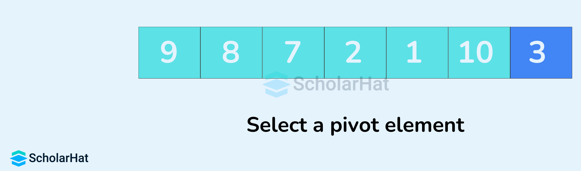
1. Pivot Selection: Choose a pivot element from the array at your convenience. For the sake of simplicity, let's assume the last element is the pivot.

   

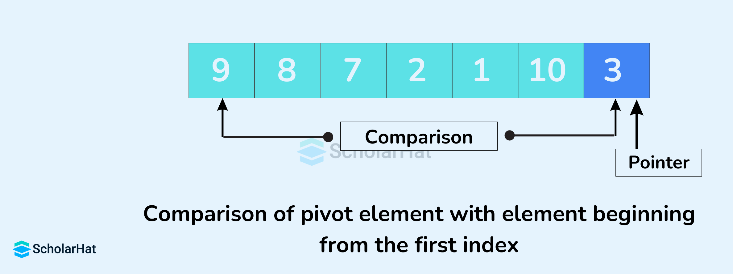
2. Partitioning: Rearrange the array such that all elements less than the pivot are placed before it, and all elements greater than the pivot are placed after it.

   

   Here's how we rearrange the array:

   1. A pointer is fixed at the pivot element. The pivot element is compared with the elements beginning from the first index.

      

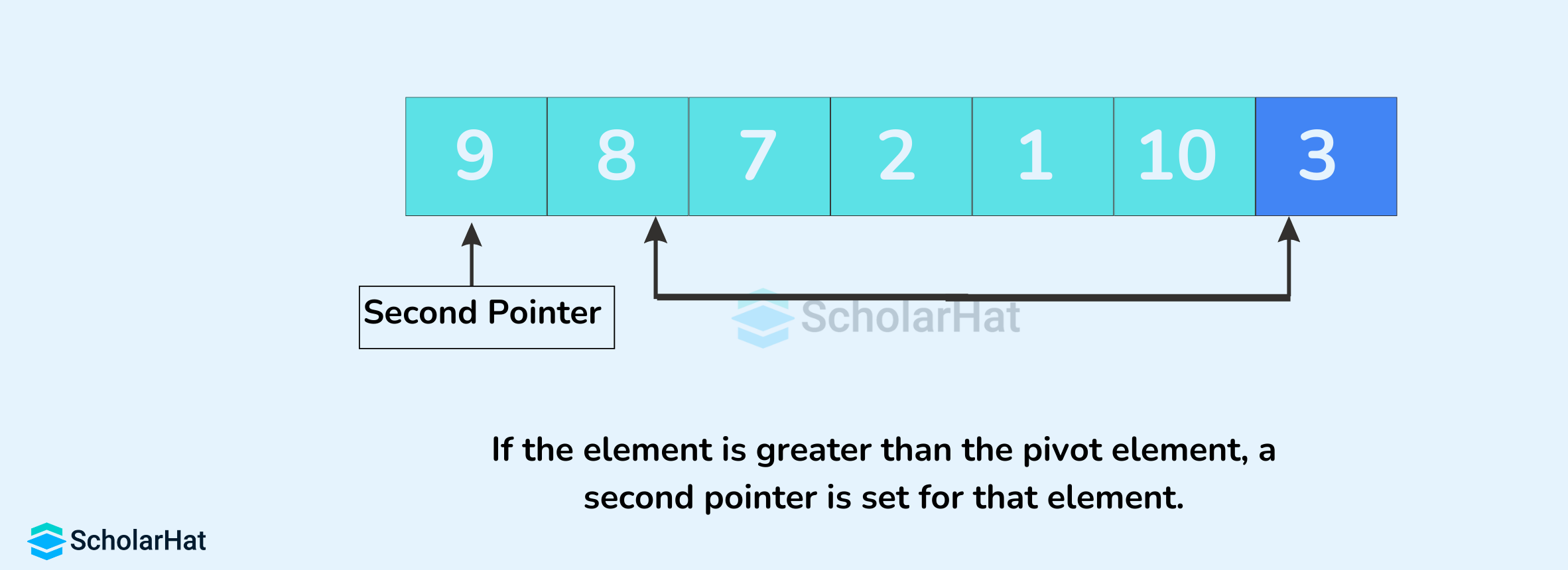
   2. If the element is greater than the pivot element, a second pointer is set for that element.

      

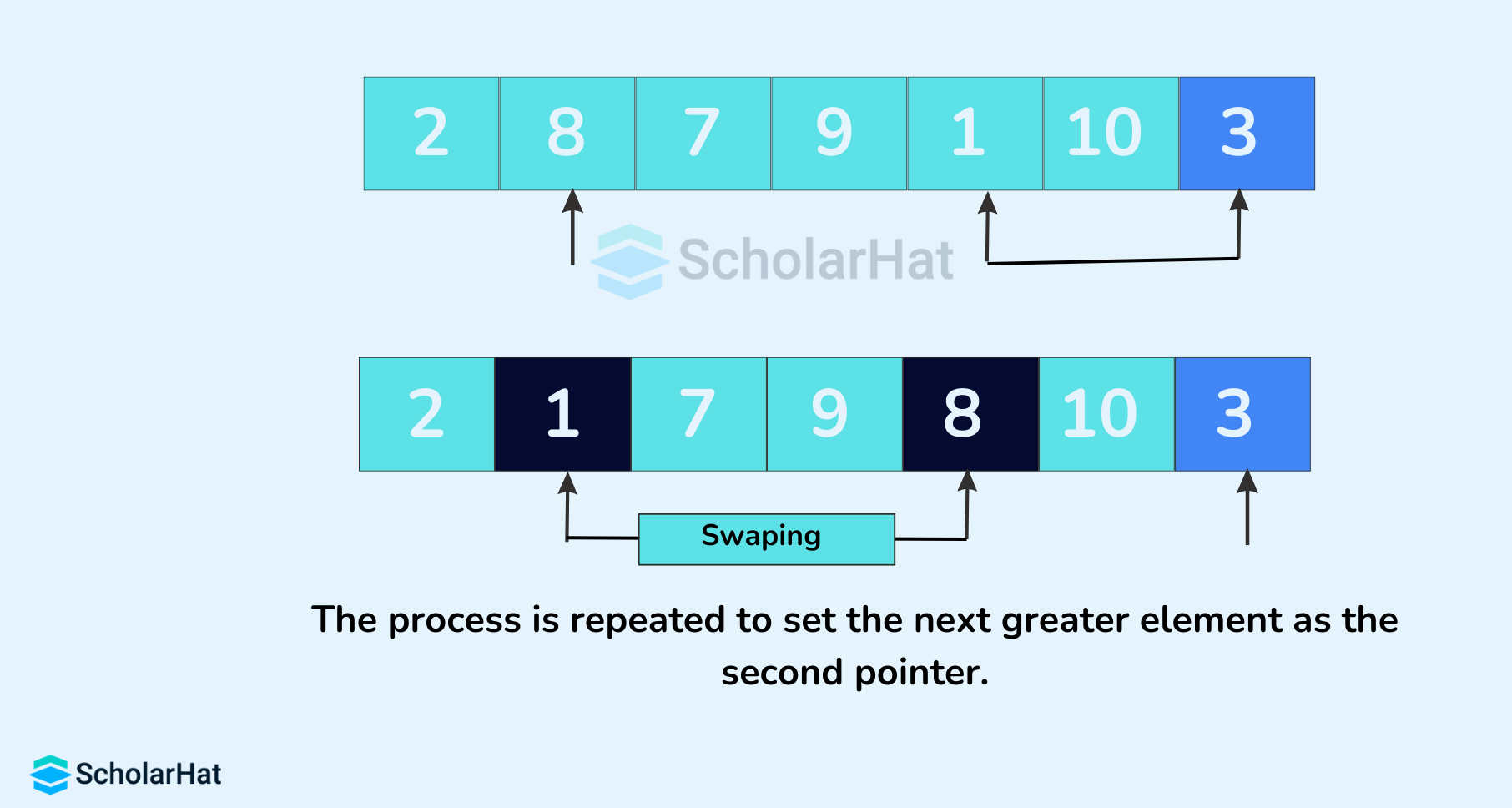
   3. Now, pivot is compared with other elements. If an element smaller than the pivot element is reached, the smaller element is swapped with the greater element found earlier.

      

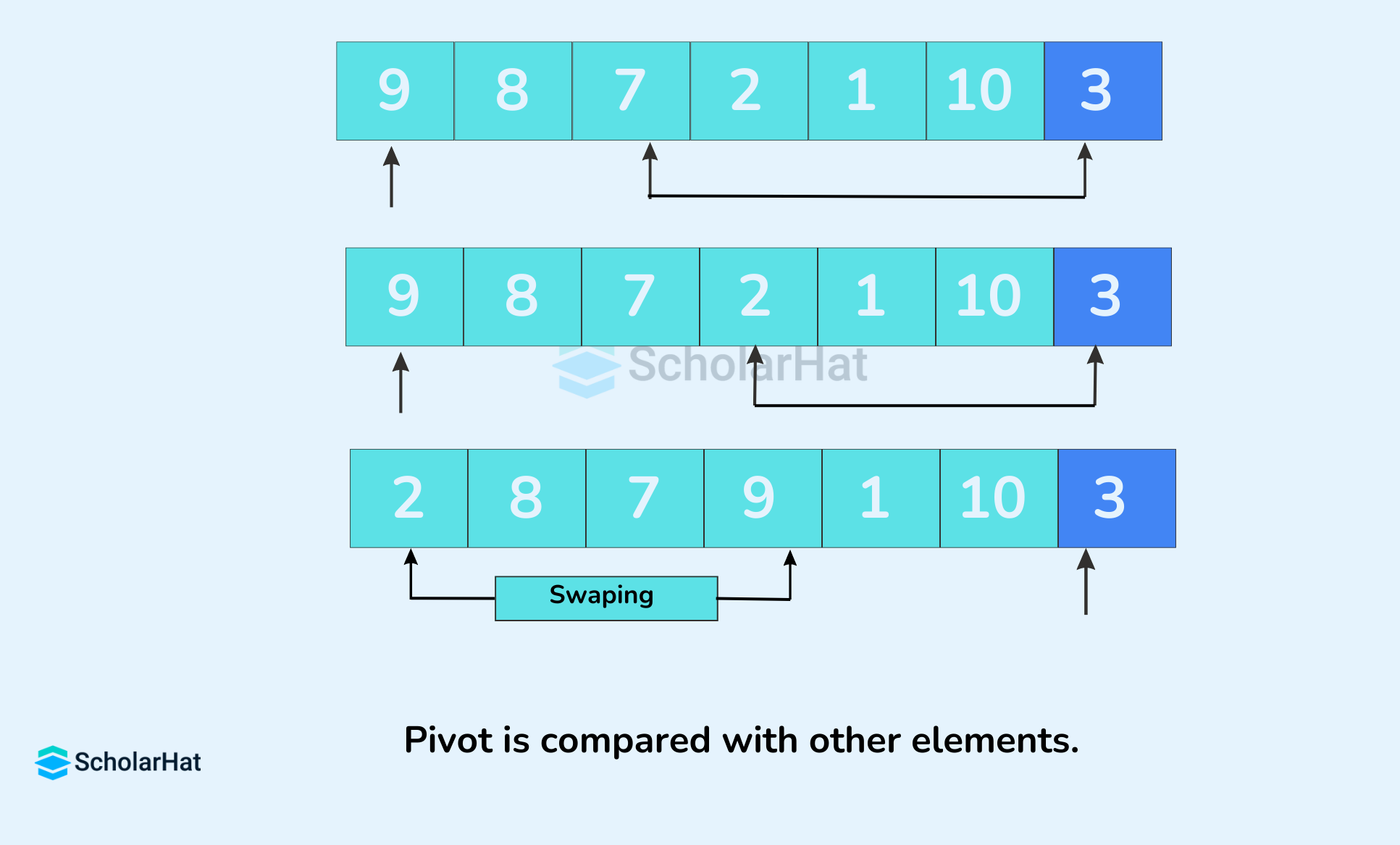
   4. Again, the process is repeated to set the next greater element as the second pointer. And, swap it with another smaller element.

      

   5. The process goes on until the second last element is reached.

      

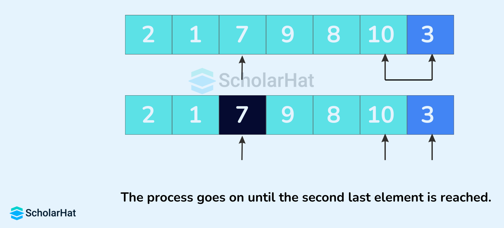
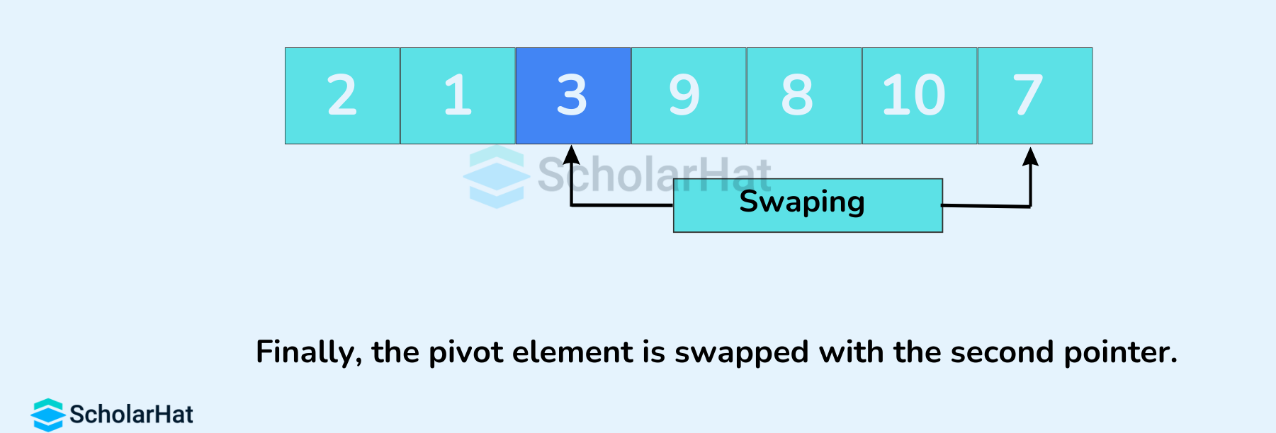
   6. Finally, the pivot element is swapped with the second pointer.

   

3. Divide Subarrays

   

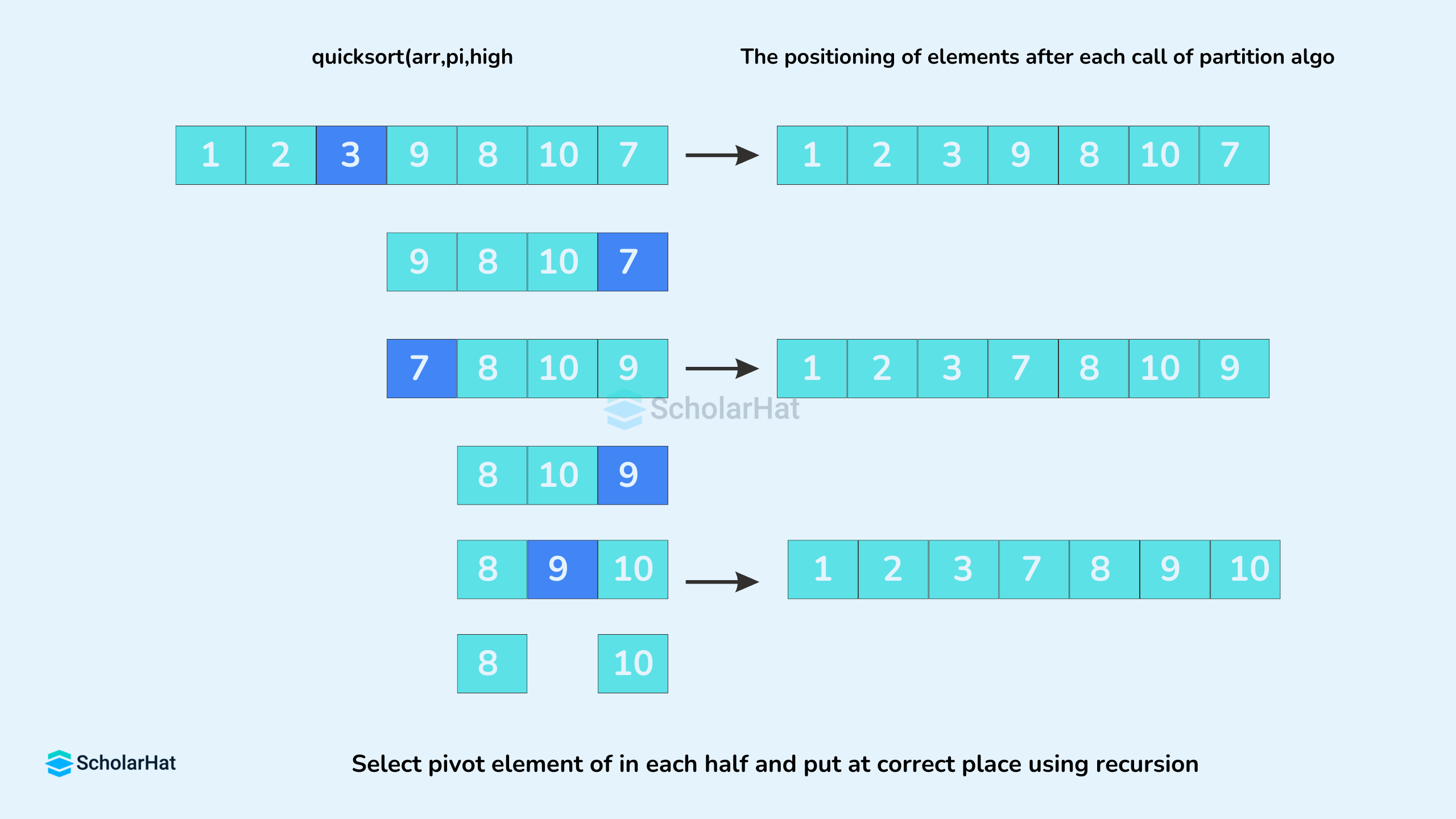
The subarrays are divided until each subarray is formed of a single element. At this point, the array is already sorted.

Read More - Data Structure Interview Questions for Freshers

Implementation of Quick Sort in Different Languages in Data Structures

# Function to find the partition position
def partition(array, low, high):
    # Choose the rightmost element as pivot
    pivot = array[high]
    # Pointer for greater element
    i = low - 1

    # Traverse through all elements
    # Compare each element with pivot
    for j in range(low, high):
        if array[j] <= pivot:
            # If element smaller than pivot is found
            # Swap it with the greater element pointed by i
            i = i + 1
            # Swapping element at i with element at j
            array[i], array[j] = array[j], array[i]

    # Swap the pivot element with the greater element specified by i
    array[i + 1], array[high] = array[high], array[i + 1]

    # Return the position from where partition is done
    return i + 1

# Function to perform quicksort
def quickSort(array, low, high):
    if low < high:
        # Find pivot element such that
        # Elements smaller than pivot are on the left
        # Elements greater than pivot are on the right
        pi = partition(array, low, high)

        # Recursive call on the left of pivot
        quickSort(array, low, pi - 1)
        # Recursive call on the right of pivot
        quickSort(array, pi + 1, high)

def print_list(arr):
    for i in range(len(arr)):
        print(arr[i], end=" ")
    print()
    
arr = [7, 2, 1, 6, 8, 5, 3, 4]
print("Original array is:", end=" ")
print_list(arr)

size = len(arr)
quickSort(arr, 0, size - 1)

print('Sorted Array in Ascending Order:', end=" ")
print_list(arr)
    

public class QuickSort {

    // Function to find the partition position
    static int partition(int[] array, int low, int high) {
        // Choose the rightmost element as pivot
        int pivot = array[high];
        // Pointer for greater element
        int i = low - 1;

        // Traverse through all elements
        // Compare each element with pivot
        for (int j = low; j < high; ++j) {
            if (array[j] <= pivot) {
                // If element smaller than pivot is found
                // Swap it with the greater element pointed by i
                i = i + 1;
                // Swapping element at i with element at j
                int temp = array[i];
                array[i] = array[j];
                array[j] = temp;
            }
        }

        // Swap the pivot element with the greater element specified by i
        int temp = array[i + 1];
        array[i + 1] = array[high];
        array[high] = temp;

        // Return the position from where partition is done
        return i + 1;
    }

    // Function to perform quicksort
    static void quickSort(int[] array, int low, int high) {
        if (low < high) {
            // Find pivot element such that
            // Elements smaller than pivot are on the left
            // Elements greater than pivot are on the right
            int pi = partition(array, low, high);

            // Recursive call on the left of pivot
            quickSort(array, low, pi - 1);
            // Recursive call on the right of pivot
            quickSort(array, pi + 1, high);
        }
    }

    public static void main(String[] args) {
        int[] arr = {7, 2, 1, 6, 8, 5, 3, 4};
        System.out.print("Original array is: ");
        for (int i : arr) {
            System.out.print(i + " ");
        }
        System.out.println();

        int size = arr.length;
        quickSort(arr, 0, size - 1);

        System.out.print("Sorted Array in Ascending Order: ");
        for (int i : arr) {
            System.out.print(i + " ");
        }
        System.out.println();
    }
}
    

#include <iostream>
using namespace std;

// function to swap elements
void swap(int *a, int *b) {
  int t = *a;
  *a = *b;
  *b = t;
}

// function to print the array
void printArray(int array[], int size) {
  int i;
  for (i = 0; i < size; i++)
    cout << array[i] << " ";
  cout << endl;
}

// function to rearrange array (find the partition point)
int partition(int array[], int low, int high) {
    
  // select the rightmost element as pivot
  int pivot = array[high];
  
  // pointer for greater element
  int i = (low - 1);

  // traverse each element of the array
  // compare them with the pivot
  for (int j = low; j < high; j++) {
    if (array[j] <= pivot) {
        
      // if element smaller than pivot is found
      // swap it with the greater element pointed by i
      i++;
      
      // swap element at i with element at j
      swap(&array[i], &array[j]);
    }
  }
  
  // swap pivot with the greater element at i
  swap(&array[i + 1], &array[high]);
  
  // return the partition point
  return (i + 1);
}

void quickSort(int array[], int low, int high) {
  if (low < high) {
      
    // find the pivot element such that
    // elements smaller than pivot are on left of pivot
    // elements greater than pivot are on righ of pivot
    int pi = partition(array, low, high);

    // recursive call on the left of pivot
    quickSort(array, low, pi - 1);

    // recursive call on the right of pivot
    quickSort(array, pi + 1, high);
  }
}

// Driver code
int main() {
  int arr[] = {7, 2, 1, 6, 8, 5, 3, 4};
  int n = sizeof(arr) / sizeof(arr[0]);
  
  cout << "Original array is: ";
  printArray(arr, n);
  
  // perform quicksort on data
  quickSort(arr, 0, n - 1);
  
  cout << "Sorted Array in Ascending Order: ";
  printArray(arr, n);
}
    

Output

Original array is: 7 2 1 6 8 5 3 4 
Sorted Array in Ascending Order: 1 2 3 4 5 6 7 8 

Complexity Analysis of Quick Sort Algorithm

1. Time complexity

   Case	Time Complexity
   Best	O(nlogn)
   Average	O(nlogn)
   Worst	O(n^2)

2. Space complexity: In the worst case, the space complexity is O(n) because here, n recursive calls are made. And, the average space complexity of a quick sort algorithm is equal to O(logn).

Applications of Quick Sort Algorithm

1. Numerical analysis:For accuracy in calculations most of the efficiently developed algorithm uses a priority queue and quick sort is used for sorting.
2. Call Optimization: It is tail-recursive and hence all the call optimization can be done.
3. Database management: Quicksort is the fastest algorithm so it is widely used as a better way of searching.

Advantages of Quick Sort Algorithm

1. Efficiency: It is efficient on large data sets.
2. In-place sorting: Quick sort performs in-place sorting, meaning it doesn't require additional memory to store temporary data or intermediate results.
3. Simple implementation: Quick sort's algorithmic logic is relatively straightforward, making it easier to understand and implement compared to some other complex sorting algorithms

Disadvantages of the Quick Sort Algorithm

1. Unstable Sorting: Quick sort is an unstable sorting algorithm, meaning that it does not guarantee the relative order of equal elements after the sorting process.
2. Worst-case Performance: Its worst-case time complexity is O(n^2). It occurs when the pivot chosen is the smallest or largest element in the array, causing unbalanced partitions.
3. Dependency on Pivot Selection: The choice of pivot significantly affects the performance of quick sort. This issue is particularly prominent when dealing with already sorted or nearly sorted arrays.
4. Recursive Overhead: Recursive function calls consume additional memory and can lead to stack overflow errors when dealing with large data sets.
5. Not Adaptive: Quick sort does not take advantage of any pre-existing order or partially sorted input. This means that even if a portion of the array is already sorted, the quick sort will still perform partitioning operations on the entire array.
6. Inefficient for Small Data Sets: Quick sort has additional overhead in comparison to some simpler sorting algorithms, especially when dealing with small data sets. The recursive nature of quick sort and the constant splitting of the array can be inefficient for sorting small arrays.

Summary

In conclusion, the Quick Sort algorithm is one of the most powerful and widely used sorting techniques in data structures. Its ability to sort large datasets efficiently using the divide-and-conquer approach makes it a preferred choice in many real-world applications. Understanding the role of the pivot element and how the algorithm breaks down problems into smaller parts is key to mastering Quick Sort. With its average-case time complexity of O(n log n), it remains a reliable and effective sorting method.

So, here we saw every aspect of the quick sort algorithm in data structures. It must not have been difficult to understand if you understood Merge Sort in Data Structures properly. To apply your knowledge of merge sort algorithm, enroll in our Free Dsa Course With Certificate.

Similar Sorting Algorithms

• Insertion Sort
• Merge Sort
• Selection Sort
• Bucket Sort

Take our Datastructures skill challenge to evaluate yourself!

In less than 5 minutes, with our skill challenge, you can identify your knowledge gaps and strengths in a given skill.

GET FREE CHALLENGE